This page has moved to my new website.
On April 8, I had written a brief description of interactions in a logistic regression model. This was a supplement to a discussion of the concepts behind the logistic regression model. Another important topic in that series of explanations is the interpretation of logistic regression coefficients for categorical variables. Just like in a linear regression model, the best way to incorporate categorical variables is to use a 0-1 coding.
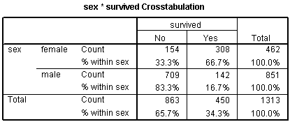
Let's start with some data that listed survival outcomes on the Titanic. That ship was struck by an iceberg and 863 passengers died out of a total of 1,313. This happened during an era where there was a strong belief in "women and children" first.

You can see this in the crosstabulation shown above. Among females, the odds of dying were 2-1 against, because the number of survivors (308) was twice as big as the number who died (154). Among males, the odds of dying were almost 5 to 1 in favor (actually 4.993 to 1), since the number who survived (142) was about one-fifth the number who died (709).
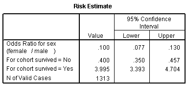
The odds ratio is 0.1, and we are very confident that this odds ratio is less than one, because the confidence interval goes up to only 0.13. Let's analyze this data by creating an indicator variable for sex.
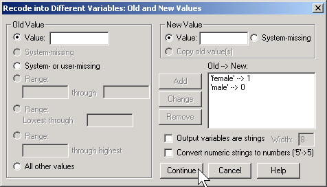
In SPSS, you would do this by selecting TRANSFORM | RECODE from the menu
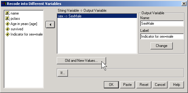
Then click on the OLD AND NEW VALUES button.
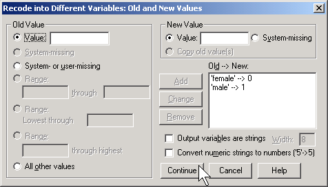
Here, I use the codes of 0 for female and 1 for male. To run a logistic regression in SPSS, select ANALYZE | REGRESSION | BINARY LOGISTIC from the menu.
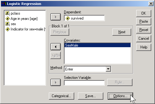
Click on the OPTIONS button.
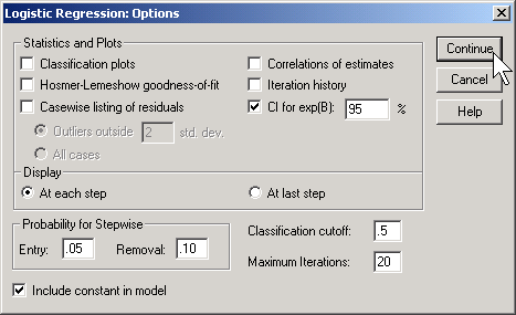
Select the CI for exp(B) option, then click on the CONTINUE button and then on the OK button. Here is what the output looks like:

Let's start with the CONSTANT row of the data. This has an interpretation similar to the intercept in the linear regression model. the B column represents the estimated log odds when SexMale=0. Above, you saw that the odds for dying were 2 to 1 against for females, and the natural logarithm of 2 is 0.693. The last column, EXP(B) represents the odds, or 2.000. You need to be careful with this interpretation, because sometimes SPSS will report the odds in favor of an event and sometimes it will report the odds against an event. You have to look at the crosstabulation to be sure which it is.
The SexMale row has an interpretation similar to the slope term in a linear regression model. The B column represents the estimated change in the log odds when SexMale increases by one unit. This is effectively the log odds ratio. We computed the odds ratio above, and -2.301 is the natural logarithm of 0.1. The last column, EXP(B) provides you with the odds ratio (0.100).
Coding is very important here. Suppose you had chosen the coding for SexFamale where1=female and 0=male.
Then the output would look quite different.

The log odds is now -1.608 which represents the log odds for males. The log odds ratio is now 2.301 and the odds ratio is 9.986 (which you might want to round to 10).
SPSS will create an indicator variable for you if you click on the CATEGORICAL button in the logistic regression dialog box.
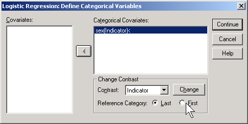
If you select LAST as the reference category, SPSS will use the code 0=male, 1=female (last means last alphabetically). If you select FIRST as the reference category, SPSS will use the code 0=female, 1=male.
How would SPSS handle a variable like Passenger Class, which has three levels
Here's a crosstabulation of survival versus passenger class.
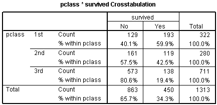
Notice that the odds of dying are 0.67 to 1 in 1st class, 1.35 to 1 in 2nd class, and 4.15 to 1 in 3rd class. These are odds in favor of dying. The odds against dying are 1.50 to 1, 0.74 to 1, and 0.24 to 1, respectively.

The odds ratio for the pclass(1) row is 6.212, which is equal to 1.50 / 0.24. You should interpret this as the odds against dying are 6 times better in first class compared to third class. The odds ratio fro the pclass(2) row is 3.069, which equals 0.74 / 0.24. This tells you that the odds against dying are about 3 times better in second class compared to third class. The Constant row tells you that the odds are 0.241 to 1 in third class.
If you prefer to do the analysis with each of the other classes being compared back to first class, then select FIRST for reference category.
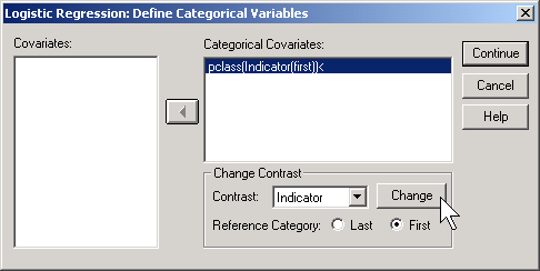
This produces the following output:

Here the pclass(1) row provides an odds ratio of 0.494 which equals 0.74 / 1.50. The odds against dying are about half in second class versus first class. The pclass(2) provides an odds ratio of 0.161 (approximately 1/6) which equals 0.24 / 1.50. The odds against dying are 1/6 in third class compared to first class. The Constant row provides an odds of 1.496 to 1 against dying for first class.
Notice that the numbers in parentheses (pclass(1) and pclass(2)) do not necessarily correspond to first and second classes. It depends on how SPSS chooses the indicator variables. How did I know how to interpret the indicator variables and the odds ratios? I wouldn't have known how to do this if I hadn't computed a crosstabulation earlier. It is very important to do a few simple crosstabulations before you run a logistic regression model, because it helps you orient yourself to the data.