The formula for uncertainty (sometimes referred to as entropy) is

By convention, if any probability is zero, we set the product term to zero as well. Those of you who are familiar with calculus could use limits to establish that zero is a reasonable value for this product.
Data compression
Consider this distribution of ratings:

The uncertainty calculation would be

Suppose we wanted to send a coded binary message that would indicate what category the rater chose. A simple approach would use three binary digits
- A=000,
- B=001,
- C=010,
- D=011,
- E=100.
to send the message. But you could use the probabilities involved to save a bit of time. Set the most common category to a shorter binary string, and longer strings to the less common categories
- A=1,
- B=000,
- C=001,
- D=010,
- E=011.
Then half of the time we would only use one bit to send the message, the other half of the time, we’d need three bits. On average, you would use two bits, which is exactly the number produced by our uncertainty calculation.
This example is a bit tricky because you might ask, why couldn’t I use two bits for B, C, D, and E. This would lead to a coding of
- A=1,
- B=00,
- C=01,
- D=10,
- E=11.
The problem with this is that unless you could separate the bits, then you couldn’t distinguish between AA (11) and E (11). You’d need a stop bit or some other type of separator, which would add to the average length of a message.
Morse code also takes advantage of probabilities, with common letters being shorter combinations of dots and dashes. The single dot and single dash are E and T, while the dot-dot, dot-dash, dash-dot, and dash-dash are I, A, N, and M, respectively. The letters that require four dots/dashes are B, C, F, H, J, L, P, Q, V, X, Y, and Z. Morse code, of course, was developed long before we understood concepts like information theory, so it is not an optimal coding. Still it represents an interesting example.
| A | B | C | D | E | F | G | H | I | J | K | L | M |
| .- | -… | -.-. | -.. | . | ..-. | –. * | *…. | ..** ** | .—** **-. | -** **.- | ..** **– | ** |
| N | O | P | Q | R | S | T | U | V | W | X | Y | Z |
| -. | — | .–. - | -.- .- | . . | .. - | .. | - …- | .– | -..- | -.– | –.. |
In general, there is not always a coding that gives the optimal number of bits on average. The uncertainty represents the lower bound on average compression rate.
Huffman encoding
One of the compression methods used by various Zip programs, Huffman encoding, takes advantage of this feature. Instead of allocating 7/8 bits to each character, it will remap the characters with the most frequently occurring characters having short bit lengths and the least frequently occurring characters having long bit lengths.
The following example appears on a rather amazing page that animates the Huffman encoding algorithm. If you were to use a simple binary coding, it would require 5 bits for each character of the alphabet A-Z. But Huffman Encoding uses a variable number of bits to represent each letter. Notice that
- E and T use 3 bits,
- A, I, L, N, O, R, and S use 4 bits,
- B, C, D, F, G, H, M, P, U, W, and Y use 5-6 bits, and
- J, K, Q, V, X and Z use 7-12 bits.


The table shows that the surprisal values are close to the number of digits used in Huffman encoding. The weighted average surprisal is 4.167, which tells us that it takes slightly more than 4 bits of information to code this data. This is confirmed by the weighted average number of bits, 4.196, which is just a tiny bit higher than the uncertainty.
Application to genetics
This is a group of DNA segments representing Lambda cI and cro binding sites.
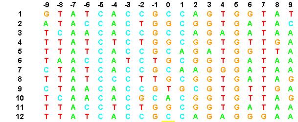
Notice that there are some common patterns to these DNA segments but also some uncertainty, especially at location zero. Information theory helps define the degree to which these DNA segments have common features.
First we need to compute the surprisal values.

If a letter has probability zero, that equals an infinite surprisal value and is dentoed by Inf in the table. Notice that letters A and G have high surprisal values in the -9 position because they only appear rarely.
The weighted surprisals appear below.

The uncertainty for this group of DNA segments is 17.5. The maximum possible uncertainty is 38 (2 bits times 19 base pairs). The information is 10.5 which represents the maximum possible uncertainty minus the uncertainty observed in this group.
One way of thinking of this is that if you knew nothing about the 19 base pair DNA segment, you would have a large amount of uncertainty (38 bits). If instead you restricted the DNA segments to the 12 listed above, you would have a lot less uncertainty. The information contained in these DNA segments represents the decrease in uncertainty.
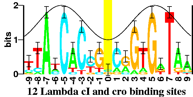
You can also compute the information at any given base pair. The information is highest at -7, -5, and +5, because these are the base pairs where there is no variation. Information is also high at -3, +3, because the probabilities of C and G respectively are almost 100%.
The following graph illustrates the information at each base pair with the heights of each letter indicating how much that particular letter contributes to the information.
Evaluating new DNA segments
There’s another way to calculate uncertainty for these DNA segments, and although it is a bit more work, it provides a clue for how to evaluate new DNA segments. Notice that for each base pair location, we have surprisal values for A, C, G, and T. We can evaluate those surprisal values for each DNA segment.
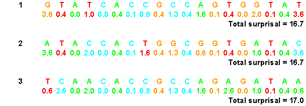
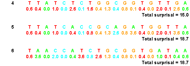
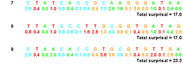
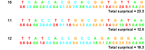
Now we can average these values across all 12 DNA segments. This gives us the same weighted surprisals and the same uncertainty as before.

This could help us understand whether one or more of the DNA segments does not fit in with the others, but more importantly, it can help us identify new DNA segments that might fit into the same class of binding sites. If a DNA segment has a reasonably low total surprisal, then that indicates that this DNA segment might fit in, but if the surprisal is too high, then this DNA segment is too different to be in this class of binding sites.
Information theory applied to sperm morphology classifications
One of the more fascinating applications of information theory is in the study of sperm morphology, the classification of sperm cells into various size and shape categories.
Human sperm exist in many different shapes and sizes. There are many irregular and abnormal forms. Forms display continuous variation and there are lots of gradual transitions from one form to another. As a result, sperm morphology has greater inter- and intra-laboratory variation than many other tests.
Although sperm morphology is a tool used in fertility assessment, fertility is a complex process that involves multiple organs of both the male and the female. Given this complexity, it would be a mistake to think that a sperm analysis is going to be a valid maker of fertility. Instead, semen analysis is a “gateway” test for fertility. It determines the path of further testing and which partner should receive greater scrutiny.
There are many sperm morphology classification schemes, and much controversy over what to use.
A good friend of mine, Susan Rothmann has an NIH grant to review morphology classification as it is currently practiced. The long term goal of the grant is to get greater consistency within and between laboratories. The preliminary data from this grant involved the classification of 160 sperm images by 99 trained raters.
Raters were asked to evaluate
the sperm head,- the acrosome region of the head,
- the postacrosomal regions of the head,
- the sperm midpiece, and
- the sperm tail.
The following picture describes the various parts of the sperm cell:
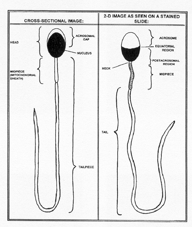
In addition, the raters were asked to classify non-sperm cells such as monocytes and macrophages that appeared in the sample. Here is a list of the classifications available in the Rothmann study:
- Head not oval (HdNOv)
- Head round (HdRnd)
- Head tapering (HdTap)
- Head pyriform (HdPyr)
- Multiple heads (HdMul)
- Amorphous head (HdAmr)
- Small head (HdSml)
- Large head (HdLrg)
- Abnormal Head Ratio (HdRat)
- Acrosome large (AcLrg)
- Acrosome small (AcSml)
- Acrosome deformed (AcDef)
- Acrosome missing (AcMis)
- Postacrosomal abnormal size (PoSiz)
- Postacrosomal abnormal shape (PoShp)
- Vacuoles (Vacuo)
- Midpiece thick (MdThk)
- Midpiece very thick (MdVTh)
- Midpiece irregular (MdIrr)
- Midpiece length (MdLen)
- Midpiece bent (MdBnt)
- Midpiece missing (MdMis)
- Midpiece droplet (MdCyt)
Midpiece incorrect insertion(MdIns)- Tail coiled (TCoil)
- Tail short (TShrt)
- Tail broken (TBrok)
- Multiple tails (TMult)
- Hairpin tail (THpin)
- Tail width (TWdth)
- Tail droplet (TDrop)
- Tail bent (TBent)
- Leukocyte (Leuko)
- Polymononuclear leukocyte (P.M.N)
- Monocyte (Moncy)
- Macrophage (Mcrph)
- Immature sperm cell (Immat)
- Spermatid (Sptid)
- Spermatocyte (Spcyt)
Not every person will use every one of these abnormal categories. The list was intended to be the collection of classifications across all systems. In addition to the specific rating categories shown above, each rater was asked to provide an overall classification:
Definitely normal,- Possibly abnormal,
- Definitely abnormal, and
- Non-sperm cell.
Here are two examples of the micrographs of sperm cells that the raters were asked to evaluate.
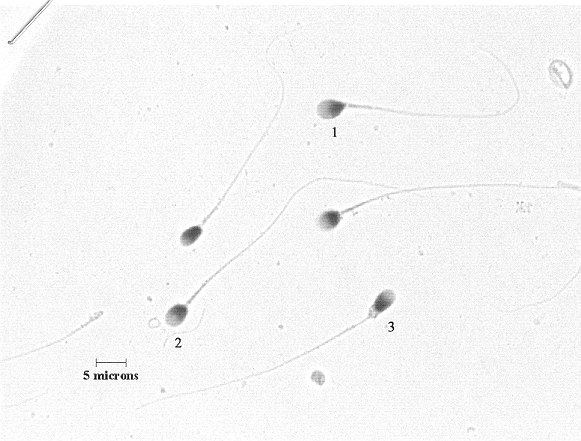
This picture and the one below it are not as good quality as the ones that the raters used, but I just wanted you to see the general type of images they were asked to rate.

What information theory can tell us about sperm classification
Certain sperm images are easier to classify and others are more difficult to classify. The former represent exemplars that can be displayed as model images of a particular classification. The latter represent areas of controversy and disagreement that need to be examined, perhaps by a consensus group, to resolve the ambiguity. Identifying the easy and difficult images is difficult by visual inspection, because of the large number of images and the variety of classifications available. We plan to use uncertainty to sift through those images and rapidly identify images both easy and difficult for further study.
Uncertainty for overall classification
The table below shows the overall classification and the uncertainty calculated on that classification.
| Cell | Norm | Bord | Abno | NonS | NotC | Unce |
| 1 | 24 | 34 | 41 | 0 | 0 | 1.6 |
| 7 | 62 | 18 | 19 | 0 | 0 | 1.3 |
| 2 | 79 | 12 | 7 | 1 | 0 | 1.0 |
| 5 | 13 | 8 | 78 | 0 | 0 | 0.9 |
| 3 | 4 | 10 | 85 | 0 | 0 | 0.7 |
| 4 | 0 | 5 | 94 | 0 | 0 | 0.3 |
| 6 | 1 | 2 | 96 | 0 | 0 | 0.2 |
The first column identifies the particular cell, and the possible classifications are abbreviated as
- Norm (Definitely normal)
- Bord (Borderline abnormal)
- Abno (Definitely abnormal)
- NonS (Non-Sperm Cell)
- NotC (Not Classified)
and “Entr” represents the calculated uncertainty. The cell with the greatest uncertainty (among the first seven cells) is cell #1. You can see by the rater counts that there was very little agreement about the overall classification of this cell.
The two cells with the least uncertainty are cells 4 and 6, and these are cells that pretty much everyone agrees are abnormal.
Information theory for individual classification
It is also possible to calculate uncertainty for each individual classification and then add these uncertainty values together. Cells with high total uncertainty represent cells with uncertainty across several classification categories. Here are the results for the first seven sperm cells with the percentages shown for any category selected by 5% or more of the raters:
Sperm #6. Uncertainty = 8.1
- TCoil: 53%
- TShrt: 44%
- MdThk: 31%
- MdVTh: 23%
- THpin: 17%
- MdLen: 13%
- MdIrr: 11%
- TWdth: 10%
- HdNOv: 8%
- HdPyr: 6%
Sperm #5. Uncertainty = 7.6
- Vacuo: 57%
- HdNOv: 32%
- HdRnd: 25%
- THpin: 20%
- AcSml: 12%
- HdSml: 11%
- HdRat: 10%
- TCoil: 9%
Sperm #3. Uncertainty = 6.4
- MdCyt: 64%
- HdNOv: 17%
- MdIrr: 16%
- HdTap: 14%
- MdVTh: 10%
- AcSml: 10%
- HdRat: 9%
- HdSml: 9%
- MdThk: 7%
- HdPyr: 5%
Sperm #1. Uncertainty = 5.8
- HdNOv: 33%
- HdPyr: 29%
- PoShp: 14%
- MdIns: 9%
- MdThk: 9%
- HdLrg: 9%
- HdRat: 8%
- HdRnd: 7%
- HdTap: 6%
Sperm #4. Uncertainty = 5.2
MdVTh: 58%MdCyt: 52%HdNOv: 12%MdIrr: 9%HdLrg: 7%HdRat: 6%
Sperm #7. Uncertainty = 2.4
TBrok: 10%TShrt: 9%HdNOv: 7%
Sperm #2. Uncertainty = 1.7
- HdNOv: 8%
Notice that cell #6, the cell with the lowest uncertainty on the overall classification, has the highest uncertainty among the seven cells when looking at the individual classification levels. This reflects the fact that raters agree that the cell is abnormal, but they can’t agree on the type of abnormality.
Future work–joint and conditional uncertainty
To calculate the total uncertainty in the sperm classification system above, I oversimplified a bit by adding the individual entropies for each individual classification system. This ignores some possibly important information. Let’s suppose that we have a two classifications: Small head (HdSml) and Missing Acrosome (AcMis). Let’s suppose there is a high amount of uncertainty in both categories:
| Y | es N | o |
| HdSml | 50% | 50% |
and
| Y | es N | o |
| AcMis | 50% | 50% |
There would be one full bit of uncertainty with each classification. But how do these classifications behave jointly? Here are two possibilities:
| Y | es N | o |
| Yes | 0% | 50% |
| No | 50% | 0% |
and
| Y | es N | o |
| Yes | 25% | 25% |
| No | 25% | 25% |
The first situation reflects a case where everyone agrees the cell is abnormal but half of the raters call it a small head and half of the raters call it a missing acrosome. The only uncertainty is in the use of labels.
The second situation is much more uncertain. A quarter of the raters say the cell has no defects, a quarter say is has two defects, and the remaining raters are split between calling the cell a small head only or a missing acrosome only.
You could calculate joint uncertainty by just treating the 2 by 2 table as a 4 by1 set of probabilities:
| Yes/Yes | Yes/No | No/Yes | No/No |
| 0% | 50% | 50% | 0% |
and
| Yes/Yes | Yes/No | No/Yes | No/No |
| 25% | 25% | 25% | 25% |
This would then allow you to calculate the joint uncertainty, and it would be 1 bit and 2 bits, respectively. The second situation, has much greater uncertainty, even though the marginal probabilities are identical to the first situation.
You can also define uncertainty using conditional probabilities, and the quantity produced, conditional uncertainty, represents how much the uncertainty in one variable is reduced when another variable is known.


There are several sperm morphology classification systems in use. Two commonly used systems are WHO-3 classification and strict classification. Strict classification works like it sounds, with borderline defects being classified as abnormal. In contrast, WHO-3 tends to classify borderline defects as normal.
Each of the 160 raters identified the system that they use. One area I want to look at is how the uncertainty decreases when you condition on rating system.
Further reading
[Coming soon!]
Acknowledgements
The Huffman coding example comes from John Morris’s web pages, in particular, http://ciips.ee.uwa.edu.au/~morris/Year2/PLDS210/huffman.html
The genetics example comes from Tom Schneider’s web site and the sequence logo graph appears on the page http://www.lecb.ncifcrf.gov/~toms/paper/trieste1996/latex/node1.html
The diagram showing the regions of the sperm cell is reproduced with permission from The Andrology Trainer, Second Edition, Donna Kinzer and Susan Rothmann. 1998. Fertility Solutions, Inc. Cleveland, OH. Page 1-8. The two micrographs of sperm cells are also reproduced with permission from Fertility Solutions, Inc.
Peter Rogan is doing some really interesting work on information theory and has inspired me to look into this more deeply. Some of his work is reflected in the software available through https://splice.cmh.edu.
You can find an earlier version of this page on my original website.