I found a larger data set and wanted to show how you could use the Kaplan Meier curves as a preliminary screen of some categorical and continuous variables in a larger and more complex data set.
I am building on a previous blog entry and this referred to an earlier webpage. Here is the R code. The comment section at the top is a cut-and-paste from the documentation of the data file.
# Some simple examples of survival analysis
# The data set is a study of primary biliary cirrhosis
# Variables:
# V1  case number
# V2  number of days between registration and the earlier of death,
# transplantion- or study analysis time in July
- 1986 # V3 status # 0=censored
- 1=censored due to liver tx
- 2=death # V4 drug # 1= D-penicillamine
- 2=placebo # V5 age in days # V6 sex # 0=male
- 1=female # V7 presence of asictes # 0=no 1=yes # V8 presence of hepatomegaly # 0=no 1=yes # V9 presence of spiders # 0=no 1=yes # V10 presence of edema
# 0 = no edema and no diuretic therapy for edema; # 0.5 = edema present without diuretics - or edema resolved by diuretics; # 1 = edema despite diuretic therapy # V11 serum bilirubin in mg/dl # V12 serum cholesterol in mg/dl # V13 albumin in gm/dl # V14 urine copper in ug/day# # V15 alkaline phosphatase in U/liter # V16 SGOT in U/ml # V17 triglicerides in mg/dl # V18 platelets per cubic ml / 1000 # V19 prothrombin time in seconds # V20 histologic stage of disease
Read the data in from the website. The first 60 rows are documentation about the file and the actual data starts on line 61.
fn <- "http://lib.stat.cmu.edu/datasets/pbc"
pbc <- read.table(fn,header=FALSE,skip=60)
head(pbc)
  V1   V2 V3 V4    V5 V6 V7 V8 V9 V10  V11 V12  V13 V14    V15    V16 V17 V18  V19 V20
1  1  400  2  1 21464  1  1  1  1 1.0 14.5 261 2.60 156 1718.0 137.95 172 190 12.2   4
2  2 4500  0  1 20617  1  0  1  1 0.0  1.1 302 4.14  54 7394.8 113.52  88 221 10.6   3
3  3 1012  2  1 25594  0  0  0  0 0.5  1.4 176 3.48 210  516.0  96.10  55 151 12.0   4
4  4 1925  2  1 19994  1  0  1  1 0.5  1.8 244 2.54  64 6121.8  60.63  92 183 10.3   4
5  5 1504  1  2 13918  1  0  1  1 0.0  3.4 279 3.53 143  671.0 113.15  72 136 10.9   3
6  6 2503  2  2 24201  1  0  1  0 0.0  0.8 248 3.98  50  944.0  93.00  63   . 11.0   3
The data looks like it read in properly - so let’s load the survival library.
> library("survival")
Loading required package: splines

Attaching package: <U+0091>survival<U+0092>

The following object is masked _by_ <U+0091>.GlobalEnv<U+0092>:

    pbc
Now that’s strange. There is an object in the survival library that has the same name (pbc). Let’s investigate.
> rm(pbc)
> head(pbc)
  id time status trt      age sex ascites hepato spiders edema bili chol albumin copper alk.phos
1  1  400      2   1 58.76523   f       1      1       1   1.0 14.5  261    2.60    156   1718.0
2  2 4500      0   1 56.44627   f       0      1       1   0.0  1.1  302    4.14     54   7394.8
3  3 1012      2   1 70.07255   m       0      0       0   0.5  1.4  176    3.48    210    516.0
4  4 1925      2   1 54.74059   f       0      1       1   0.5  1.8  244    2.54     64   6121.8
5  5 1504      1   2 38.10541   f       0      1       1   0.0  3.4  279    3.53    143    671.0
6  6 2503      2   2 66.25873   f       0      1       0   0.0  0.8  248    3.98     50    944.0
     ast trig platelet protime stage
1 137.95  172      190    12.2     4
2 113.52   88      221    10.6     3
3  96.10   55      151    12.0     4
4  60.63   92      183    10.3     4
5 113.15   72      136    10.9     3
6  93.00   63       NA    11.0     3
Wow! The data set I was importing was already part of the survival library. Let’s use their version - since it has better names for the variables than V1-V20.
We have to subset the data because the first 312 observations represent a randomized trial and the remaining observations are an add-on study of baseline values for some non-randomized patients.
> tail(pbc)
     id time status trt      age sex ascites hepato spiders edema bili chol albumin copper
413 413  989      0  NA 35.00068   f      NA     NA      NA     0  0.7   NA    3.23     NA
414 414  681      2  NA 67.00068   f      NA     NA      NA     0  1.2   NA    2.96     NA
415 415 1103      0  NA 39.00068   f      NA     NA      NA     0  0.9   NA    3.83     NA
416 416 1055      0  NA 56.99932   f      NA     NA      NA     0  1.6   NA    3.42     NA
417 417  691      0  NA 58.00137   f      NA     NA      NA     0  0.8   NA    3.75     NA
418 418  976      0  NA 52.99932   f      NA     NA      NA     0  0.7   NA    3.29     NA
    alk.phos ast trig platelet protime stage
413       NA  NA   NA      312    10.8     3
414       NA  NA   NA      174    10.9     3
415       NA  NA   NA      180    11.2     4
416       NA  NA   NA      143     9.9     3
417       NA  NA   NA      269    10.4     3
418       NA  NA   NA      350    10.6     4
> pmod <- pbc[1:312,]
> tail(pmod)
     id time status trt      age sex ascites hepato spiders edema bili chol albumin copper
307 307 1149      0   2 30.57358   f       0      0       0     0  0.8  273    3.56     52
308 308 1153      0   1 61.18275   f       0      1       0     0  0.4  246    3.58     24
309 309  994      0   2 58.29979   f       0      0       0     0  0.4  260    2.75     41
310 310  939      0   1 62.33265   f       0      0       0     0  1.7  434    3.35     39
311 311  839      0   1 37.99863   f       0      0       0     0  2.0  247    3.16     69
312 312  788      0   2 33.15264   f       0      0       1     0  6.4  576    3.79    186
    alk.phos ast trig platelet protime stage
307     1282 130   59      344    10.5     2
308      797  91  113      288    10.4     2
309     1166  70   82      231    10.8     2
310     1713 171  100      234    10.2     2
311     1050 117   88      335    10.5     2
312     2115 136  149      200    10.8     2
Take a look at the two key variables needed to define the survival object. Dividing by 365.25 gives the times in years rather than in days.
> summary(pmodtime)
   Min. 1st Qu.  Median    Mean 3rd Qu.    Max.
     41    1191    1840    2006    2697    4556
> summary(pmodtime/365.25)
   Min. 1st Qu.  Median    Mean 3rd Qu.    Max.
 0.1123  3.2610  5.0360  5.4930  7.3850 12.4700
> table(pmodstatus)

  0   1   2
168  19 125
The values for status - if you read the documentation - are 0=censored, 1=transplant - and 2=death. You could define an event as either 1 and 2 or 2 by itself. Choose the latter for this example.
> p.surv >- Surv(pmodtime,pmod$status==2)
print(p.surv)
  [1]  400  4500+ 1012  1925  1504+ 2503  1832+ 2466  2400    51  3762   304  3577+ 1217  3584
 [16] 3672+  769   131  4232+ 1356  3445+  673   264  4079  4127+ 1444    77   549  4509+  321
 [31] 3839  4523+ 3170  3933+ 2847  3611+  223  3244  2297  4467+ 1350  4453+ 4556+ 3428  4025+
 [46] 2256  2576+ 4427+  708  2598  3853  2386  1000  1434  1360  1847  3282  4459+ 2224  4365+
 [61] 4256+ 3090   859  1487  3992+ 4191  2769  4039+ 1170  3458+ 4196+ 4184+ 4190+ 1827  1191
 [76]   71   326  1690  3707+  890  2540  3574  4050+ 4032+ 3358  1657   198  2452+ 1741  2689
 [91]  460   388  3913+  750   130  3850+  611  3823+ 3820+  552  3581+ 3099+  110  3086  3092+
[106] 3222  3388+ 2583  2504+ 2105  2350+ 3445   980  3395  3422+ 3336+ 1083  2288   515  2033+
[121]  191  3297+  971  3069+ 2468+  824  3255+ 1037  3239+ 1413   850  2944+ 2796  3149+ 3150+
[136] 3098+ 2990+ 1297  2106+ 3059+ 3050+ 2419   786   943  2976+ 2615+ 2995+ 1427   762  2891+
[151] 2870+ 1152  2863+  140  2666+  853  2835+ 2475+ 1536  2772+ 2797+  186  2055   264  1077
[166] 2721+ 1682  2713+ 1212  2692+ 2574+ 2301+ 2657+ 2644+ 2624+ 1492  2609+ 2580+ 2573+ 2563+
[181] 2556+ 2555+ 2241+  974  2527+ 1576   733  2332+ 2456+ 2504+  216  2443+  797  2449+ 2330+
[196] 2363+ 2365+ 2357+ 1592+ 2318+ 2294+ 2272+ 2221+ 2090  2081  2255+ 2171+  904  2216+ 2224+
[211] 2195+ 2176+ 2178+ 1786  1080  2168+  790  2170+ 2157+ 1235  2050+  597   334  1945+ 2022+
[226] 1978+  999  1967+  348  1979+ 1165  1951+ 1932+ 1776+ 1882+ 1908+ 1882+ 1874+  694  1831+
[241]  837+ 1810+  930  1690  1790+ 1435+  732+ 1785+ 1783+ 1769+ 1457+ 1770+ 1765+  737+ 1735+
[256] 1701+ 1614+ 1702+ 1615+ 1656+ 1677+ 1666+ 1301+ 1542+ 1084+ 1614+  179  1191  1363+ 1568+
[271] 1569+ 1525+ 1558+ 1447+ 1349+ 1481+ 1434+ 1420+ 1433+ 1412+   41  1455+ 1030+ 1418+ 1401+
[286] 1408+ 1234+ 1067+  799  1363+  901+ 1329+ 1320+ 1302+  877+ 1321+  533+ 1300+ 1293+  207
[301] 1295+ 1271+ 1250+ 1230+ 1216+ 1216+ 1149+ 1153+  994+  939+  839+  788+
First - let’s look at an overall survival curve.
> plot(survfit(p.surv~1))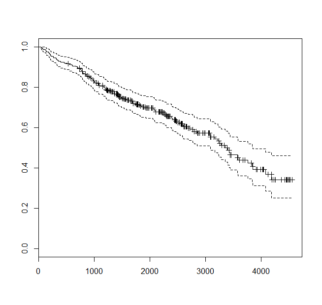
Now let’s define some functions that will calculate and compare Kaplan-Meier curves across all the possible covariates in the model. For categorical variables - draw Kaplan-Meier curves for each category level. For continuous variables - split the data into quartiles and then draw Kaplan-Meier curves for each quartile.
km.cat <- function(vn) {
print(vn)
print(table(pmod[,vn]))
km.all(pmod[,vn])
title(vn)
}
km.con <- function(vn) {
print(vn)
br <- quantile(pmod[,vn],na.rm=TRUE)
br[1] <- 0
quartiles <- cut(pmod[,vn],breaks=br)
print(table(quartiles))
km.all(quartiles)
title(vn)
}
km.all <- function(x) {
tb <- table(x)
mi <- sum(is.na(x))
sf <- survfit(p.surv~x)
print(paste("There are",mi,"missing values."))
plot(sf,xlim=c(0,6000))
end.pts <- cumsum(sfstrata)
end.x <- sftime[end.pts]+100
end.y <- sfsurv[end.pts]
end.nm <- names(tb)
text(end.x,end.y,end.nm,cex=1.5,col="darkred",adj=0)
}
v.cat <- names(pmod)[c(4,6:10,20)]
v.con <- names(pmod)[c(5,11:19)]
for (v in v.cat) {
km.cat(v)
}
for (v in v.con) {
km.con(v)
}
Here is the output.
v.cat <- names(pmod)[c(4,6:10,20)]
v.con <- names(pmod)[c(5,11:19)]
for (v in v.cat) {
  km.cat(v)
}
## [1] "trt"
##
## 1 2
## 158 154
## [1] "There are 0 missing values."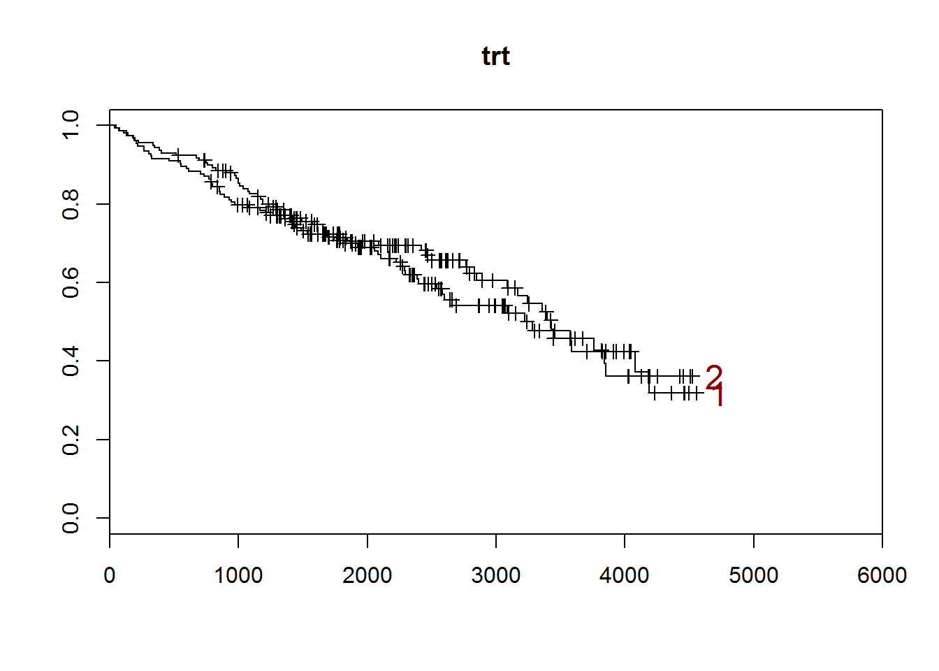
## [1] "sex"
##
##   m   f
##  36 276
## [1] "There are 0 missing values."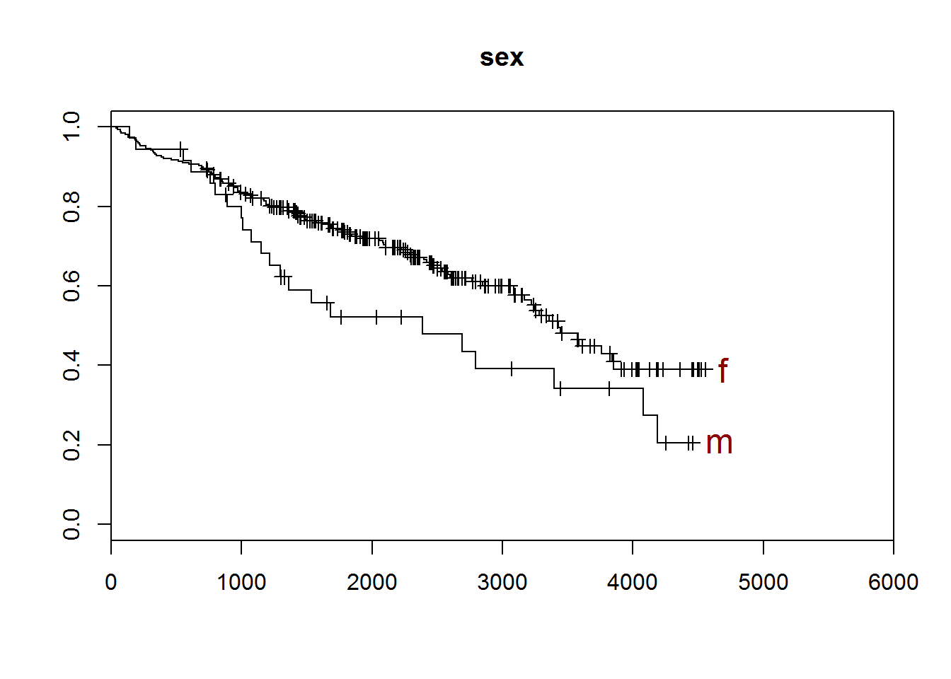
## [1] "ascites"
##
##   0   1
## 288  24
## [1] "There are 0 missing values."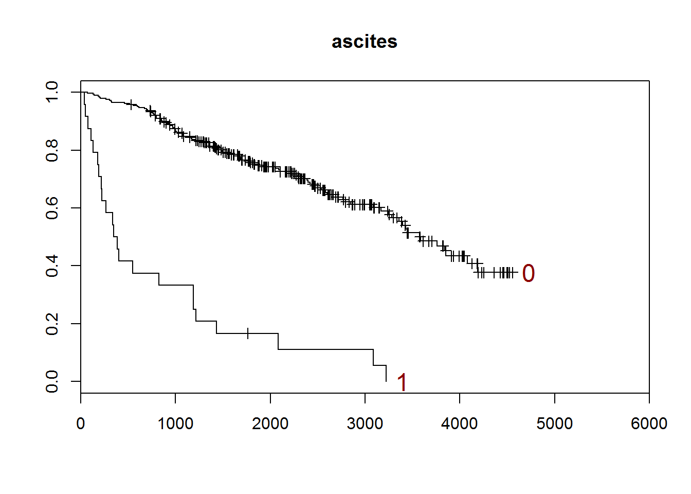
## [1] "hepato"
##
##   0   1
## 152 160
## [1] "There are 0 missing values."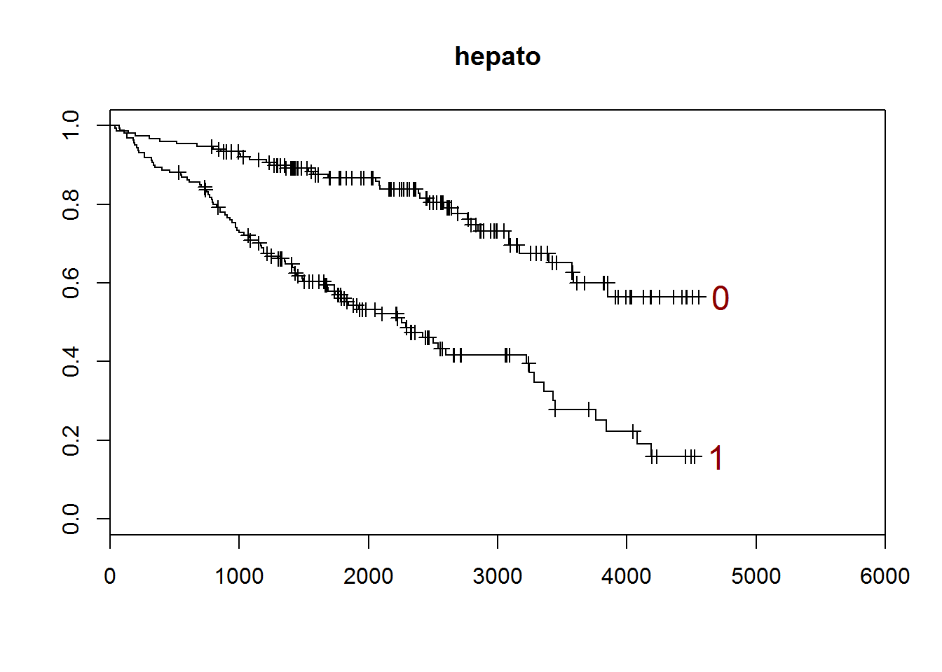
## [1] "spiders"
##
##   0   1
## 222  90
## [1] "There are 0 missing values."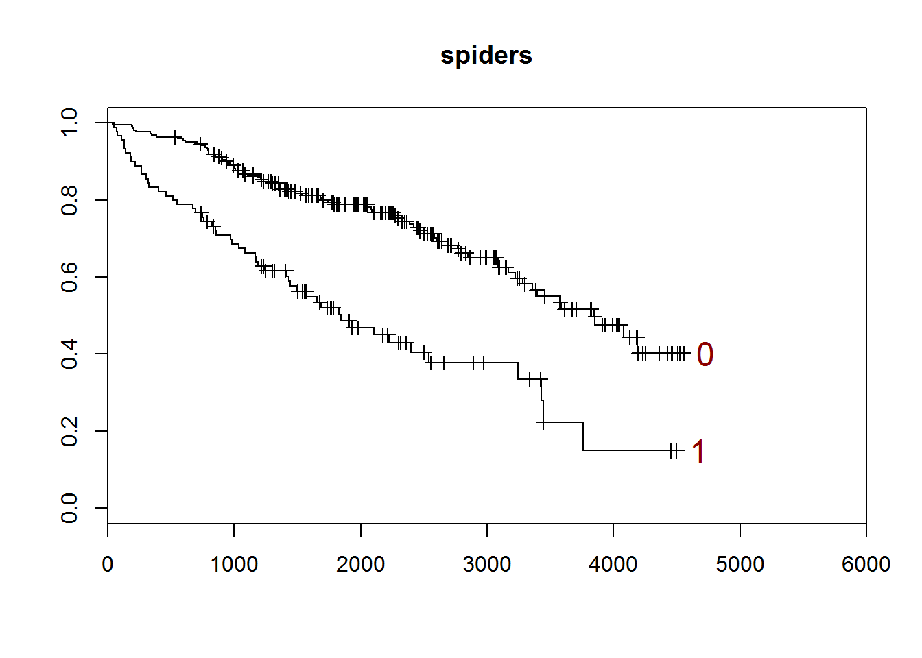
## [1] "edema"
##
##   0 0.5   1
## 263  29  20
## [1] "There are 0 missing values."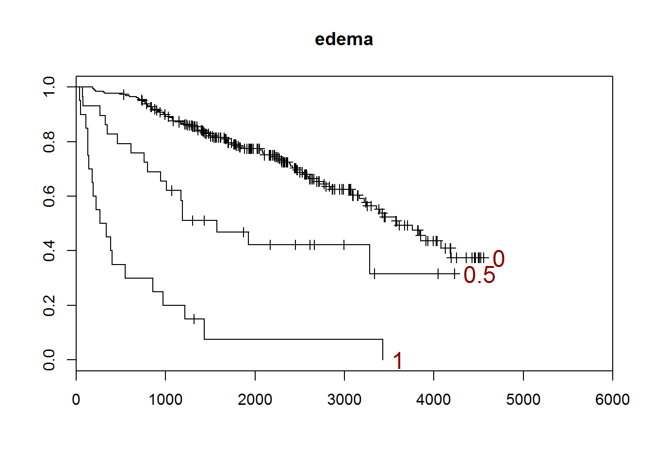
## [1] "stage"
##
##   1   2   3   4
##  16  67 120 109
## [1] "There are 0 missing values."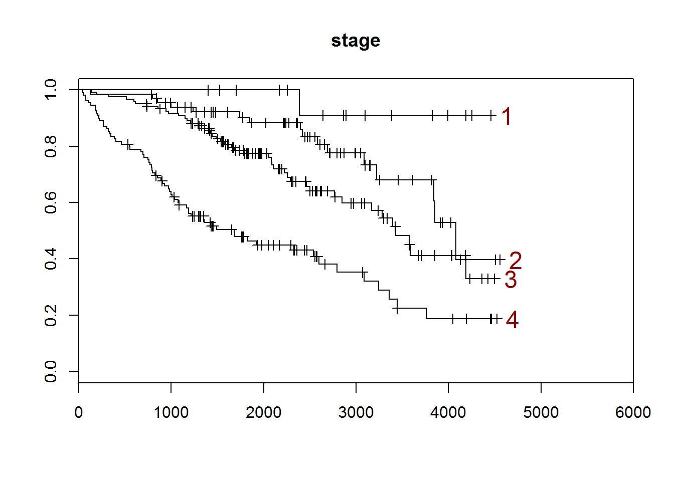
for (v in v.con) {
  km.con(v)
}
## [1] "age"
## quartiles
## (0,42.2] (42.2,49.8] (49.8,56.7] (56.7,78.4]
## 78 78 78 78
## [1] "There are 0 missing values."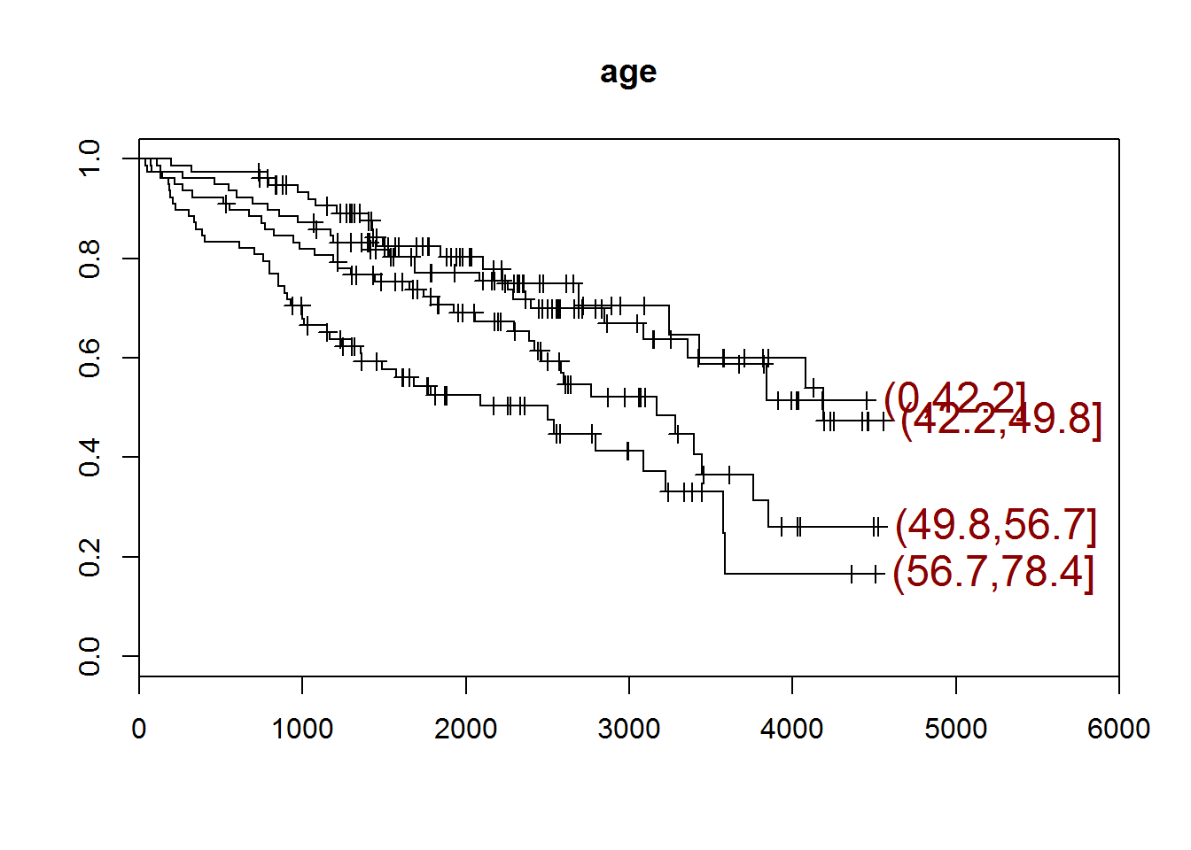
## [1] "bili"
## quartiles
##     (0,0.8]  (0.8,1.35] (1.35,3.42]   (3.42,28]
##          90          66          78          78
## [1] "There are 0 missing values."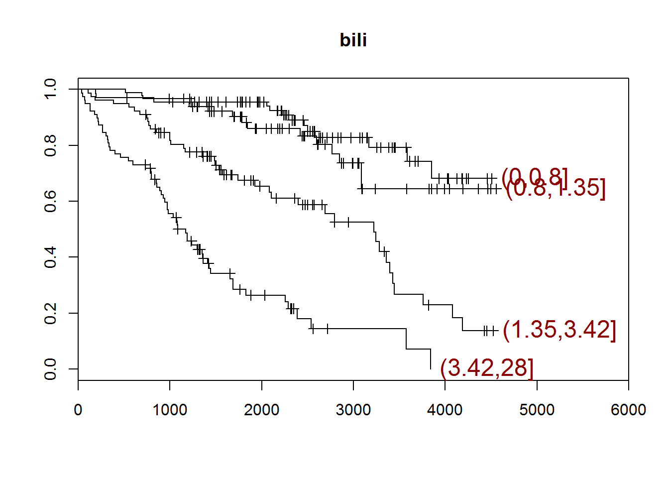
## [1] "chol"
## quartiles
##        (0,250]      (250,310]      (310,400] (400,1.78e+03]
##             71             71             72             70
## [1] "There are 28 missing values."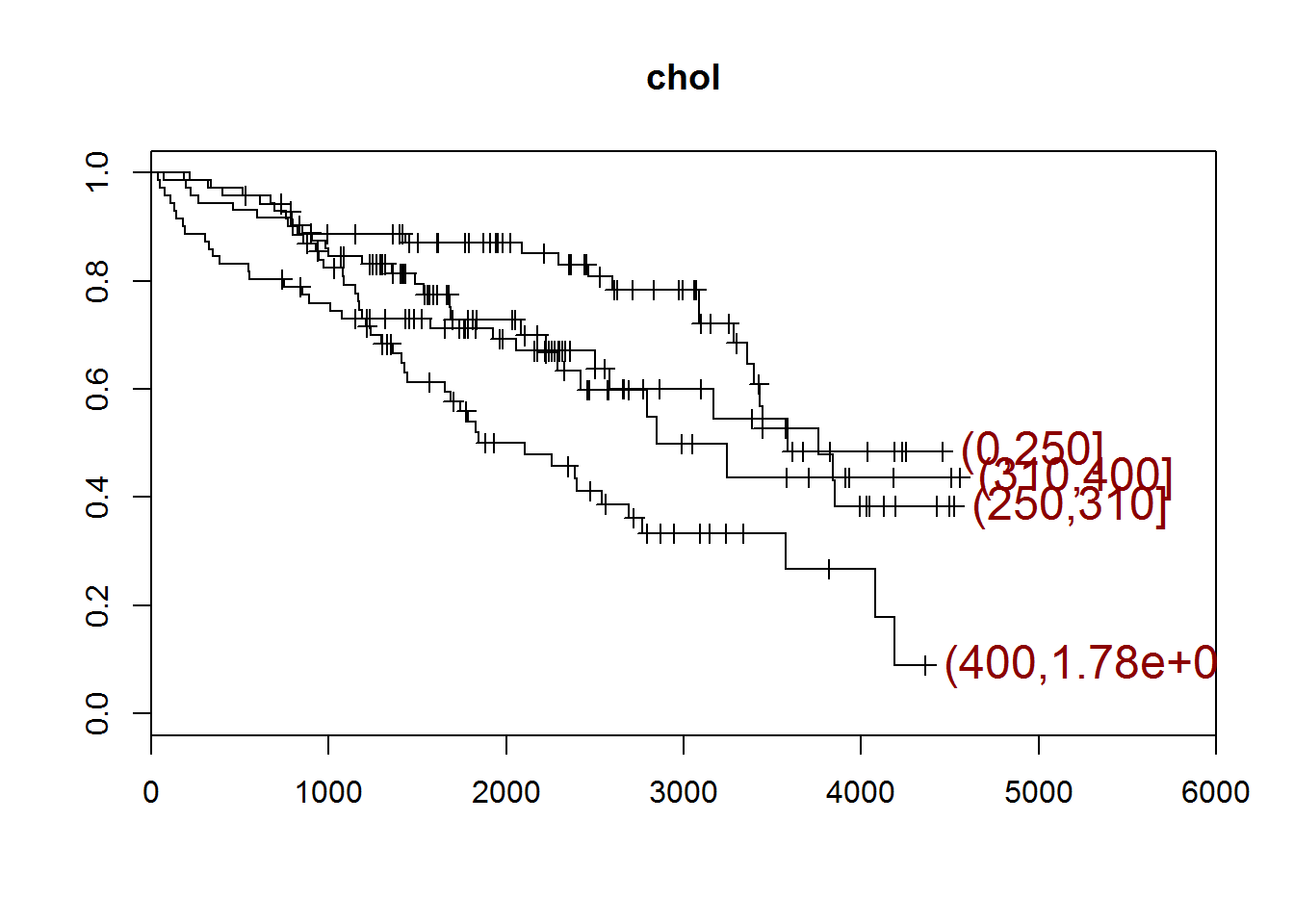
## [1] "albumin"
## quartiles
##    (0,3.31] (3.31,3.55]  (3.55,3.8]  (3.8,4.64]
##          81          76          81          74
## [1] "There are 0 missing values."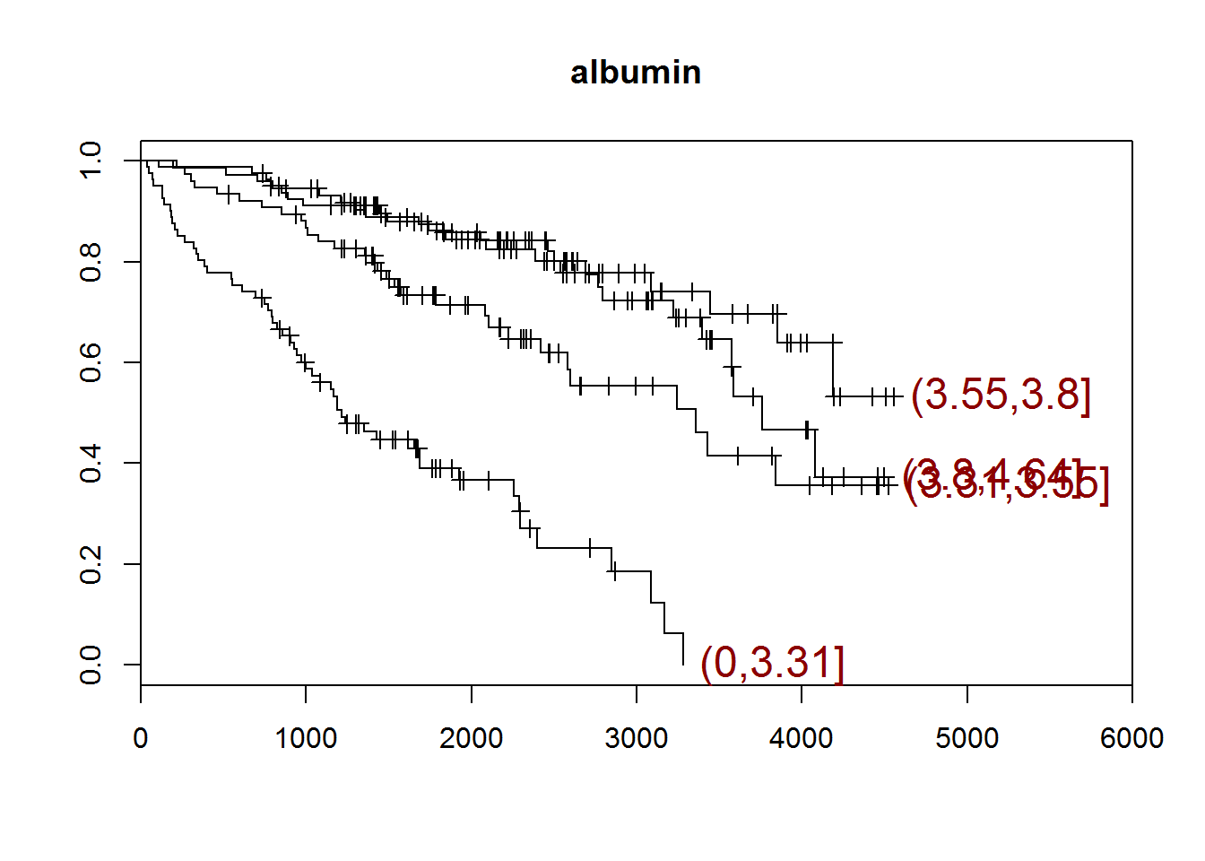
## [1] "copper"
## quartiles
##  (0,41.2] (41.2,73]  (73,123] (123,588]
##        78        80        75        77
## [1] "There are 2 missing values."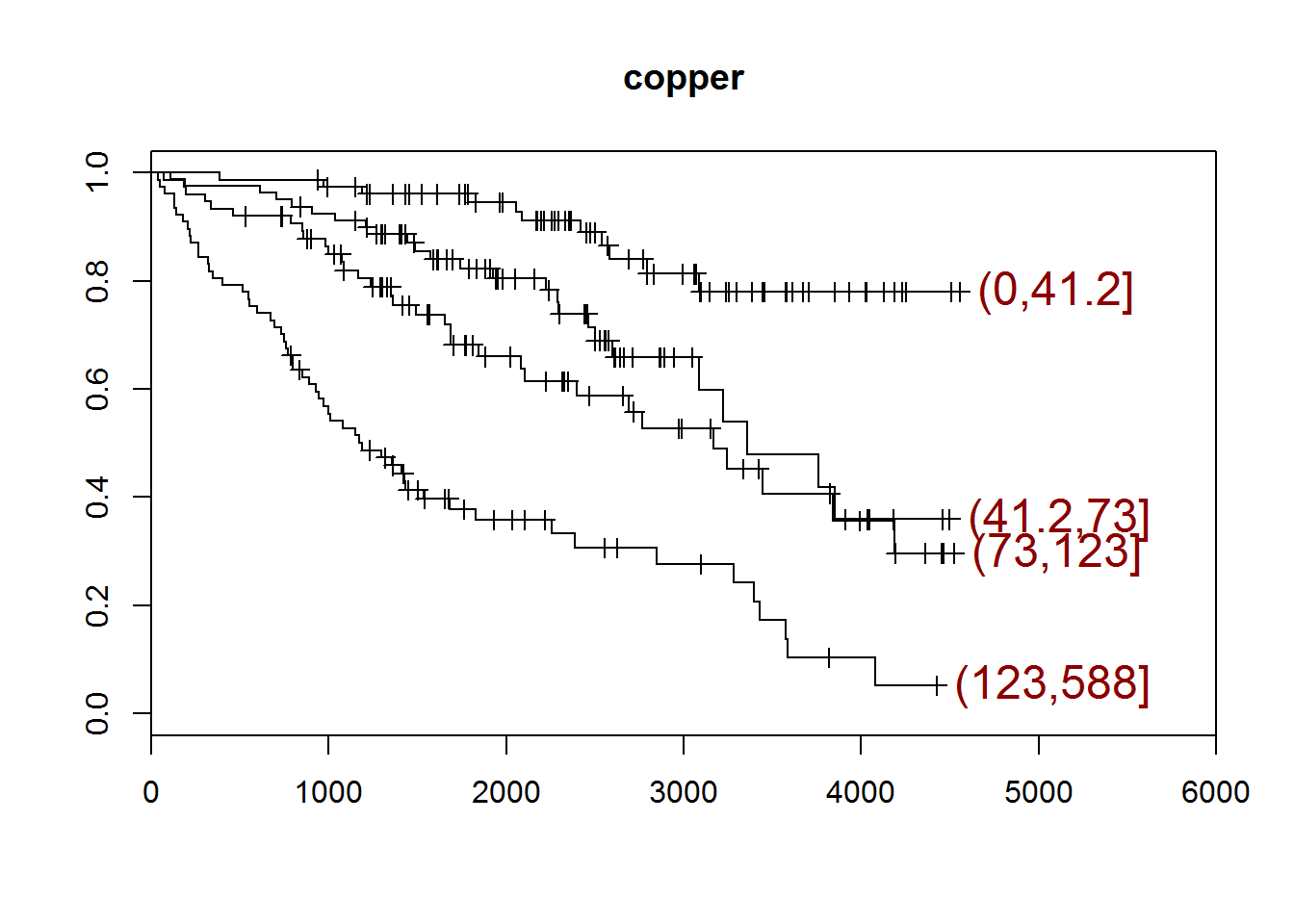
## [1] "alk.phos"
## quartiles
##             (0,872]      (872,1.26e+03] (1.26e+03,1.98e+03]
##                  78                  78                  78
## (1.98e+03,1.39e+04]
##                  78
## [1] "There are 0 missing values."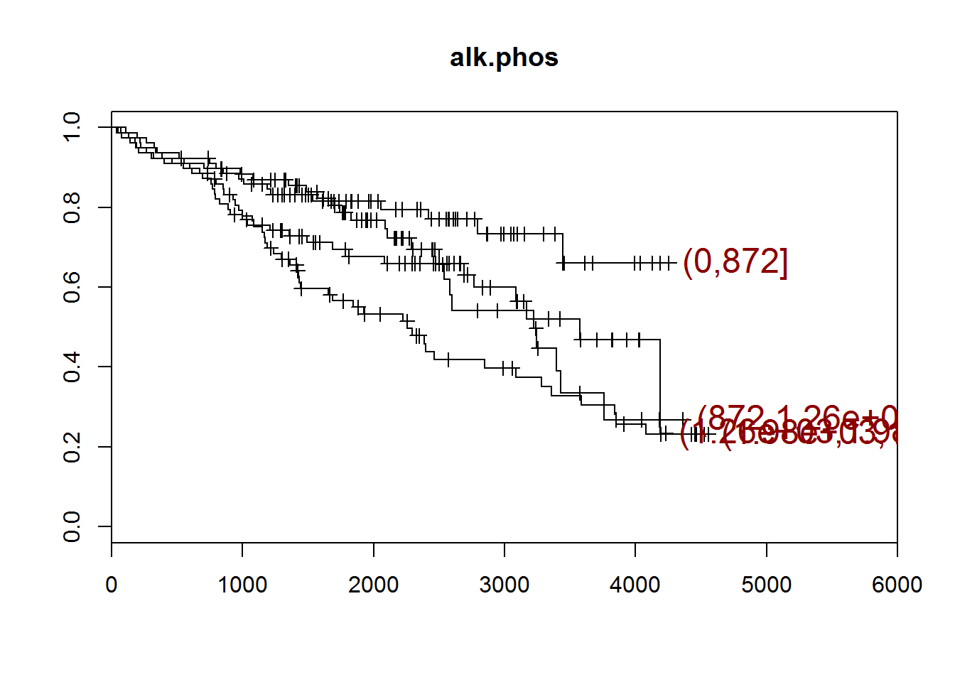
## [1] "ast"
## quartiles
##   (0,80.6] (80.6,115]  (115,152]  (152,457]
##         79         78         79         76
## [1] "There are 0 missing values."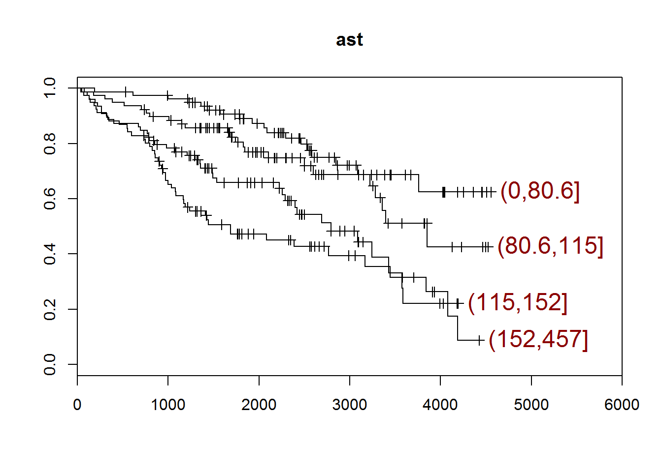
## [1] "trig"
## quartiles
##   (0,84.2] (84.2,108]  (108,151]  (151,598]
##         71         71         70         70
## [1] "There are 30 missing values."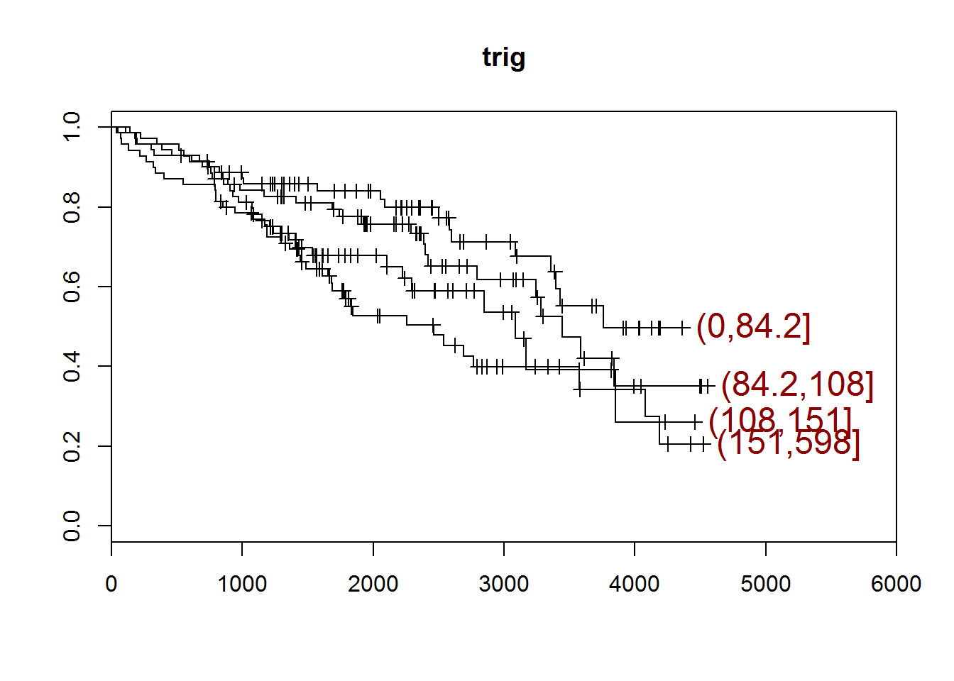
## [1] "platelet"
## quartiles
##   (0,200] (200,257] (257,322] (322,563]
##        77        77        77        77
## [1] "There are 4 missing values."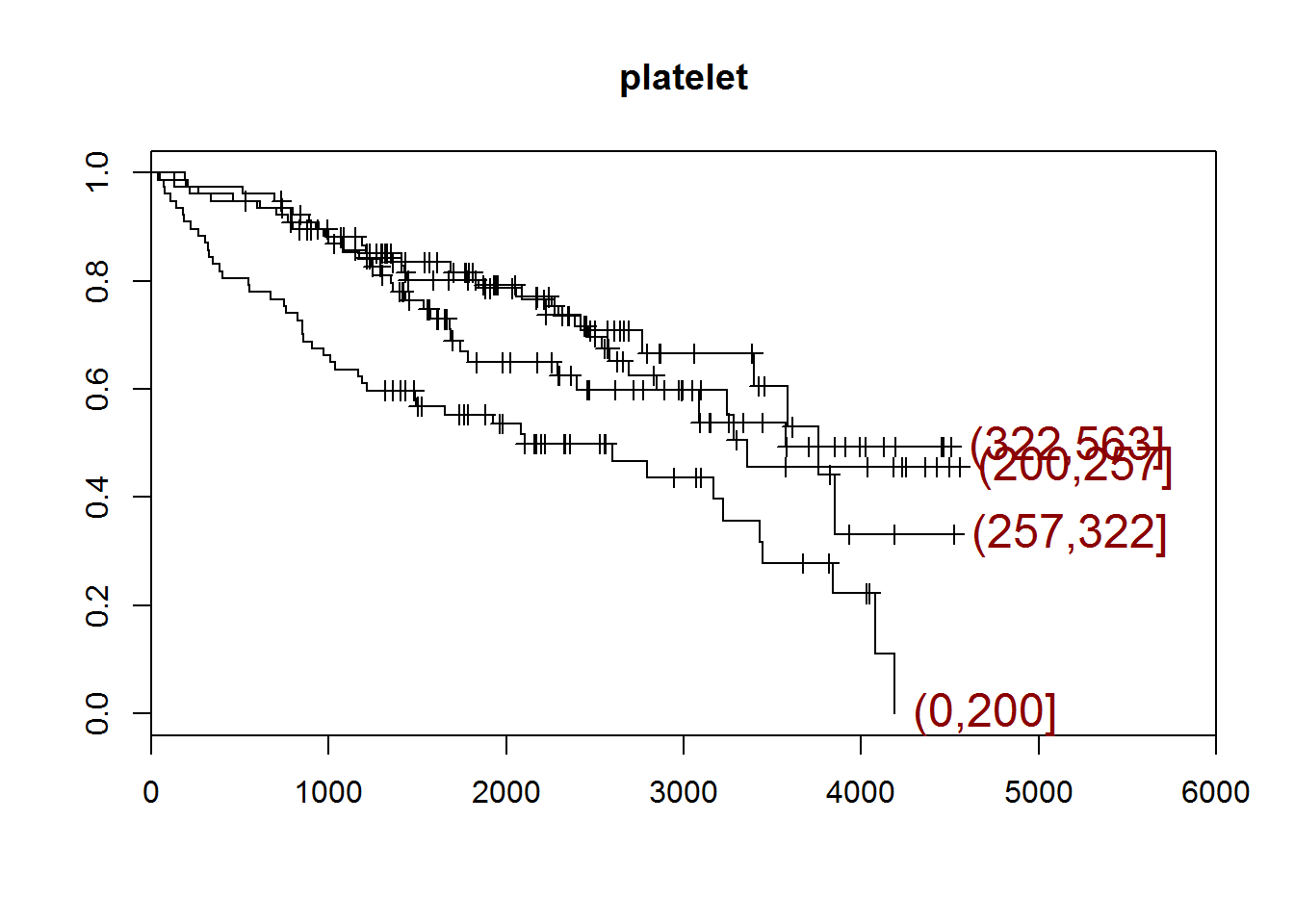
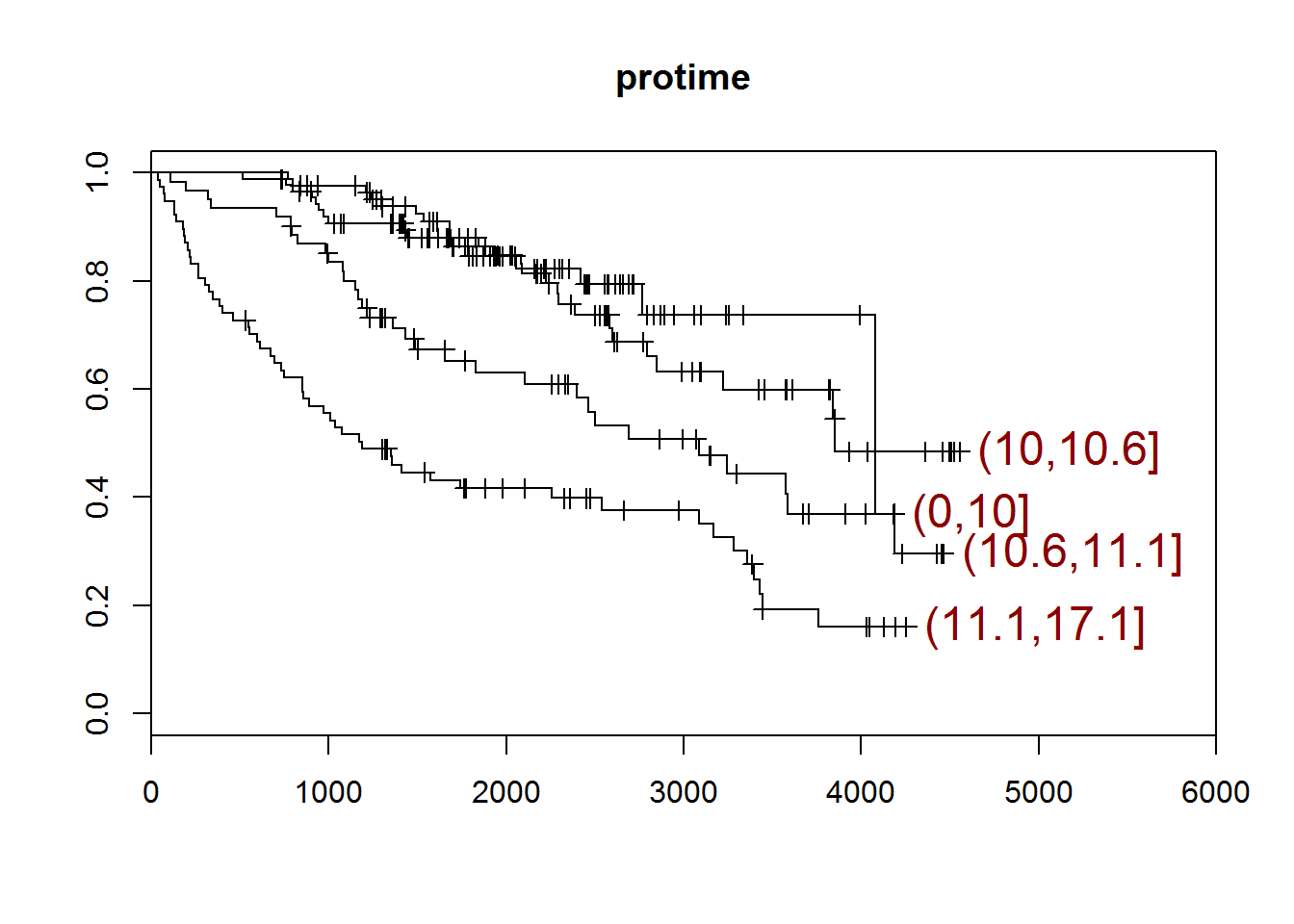
## [1] "protime"
## quartiles
##      (0,10]   (10,10.6] (10.6,11.1] (11.1,17.1]
##          89          85          61          77
## [1] "There are 0 missing values."