P.Mean >> Statistics webinar
>> P-values, confidence intervals, and the Bayesian alternative (presented 2009-09-14).
I will be hosting a free webinar (web seminar) on Wednesday, October 14, 10am-noon, CDT.
The topic is "P-values, confidence intervals, and the Bayesian alternative."
This is the handout I will use for that webinar.
I am also using this handout for a presentation to the Midwest Society for
Pediatric Research on Thursday, October 8.
Abstract: P-values and confidence intervals are the fundamental tools used
in most inferential data analyses. They are possibly the most commonly
reported statistics in the medical literature. Unfortunately, both p-values
and confidence intervals are subject to frequent misinterpretations. In this
two hour webinar, you will learn the proper interpretation of p-values and
confidence intervals, and the common abuses and misconceptions about these
statistics. You will also see a simple application of Bayesian analysis which
provides an alternative to p-values and confidence intervals.
In this seminar, you will learn how to:
- distinguish between statistical significance and clinical significance;
- define and interpret p-values;
- explain the ethical issues associated with inadequate sample sizes.
- explain the difference between informative and diffuse priors;
- interpret statistics from a posterior distribution.
If the free webinar is successful, then I will offer additional webinars for a fee. I have
developed a list of possible topics for
these webinars,
though this may change depending on feedback that I get. If you want to be notified about future webinars, the easiest way is to sign up for my newsletter, The Monthly Mean,
This newsletter will include publicity about the upcoming free webinar in the
September issue, which I'm hoping to distribute in early October and future
paid webinars in future issues. Future paid webinars will also be publicized
on the www.pmean.com website.
Here's the outline of this talk
- Icebreaker
- Pop quiz
- Definitions
- What is a p-value?
- Practice exercises
- What is a confidence interval?
- Practice exercises
- A simple example of Bayesian data analysis.
- Repeat of pop quiz
This talk is based largely on a training class that I offered at Children's
Mercy Hospital, Stats
#22 : What Do All These Numbers Mean? Confidence Intervals and P-Values,
but also includes material from Chapter 6 of my book, Statistical Evidence in Medical Trials,
and material from the lead article of the July/August issue of The Monthly Mean,
Icebreaker
In your job, you may have had to calculate a statistic of one sort or
another. It might have been a simple statistic like a mean or a percentage, it
might have been more complicated, like a correlation coefficient, or it might
have been something very difficult, like a Poisson regression model with an
overdispersion parameter. Tell us about the most complex statistic that you
have ever computed, either by hand or using a computer. Include only those
statistics that you have calculated outside of your university training. Don't
include any statistic that someone else calculated for you. Here's a list
sorted (more or less) by the complexity of the statistic.
- percentage
- mean
- standard deviation
- t-test
- correlation coefficient
- linear regression model
- survival curve
- logistic regression model
- other
By the way, you won't need knowledge or familiarity with any of the above
statistics to follow the content of this presentation. I am just trying to
gauge the experience level of my audience.
Pop quiz
A research paper computes a p-value of 0.45. How would you interpret this
p-value?
- Strong evidence for the null hypothesis
- Strong evidence for the alternative hypothesis
- Little or no evidence for the null hypothesis
- Little or no evidence for the alternative hypothesis
- More than one answer above is correct.
- I do not know the answer.
A research paper computes a confidence interval for a relative risk of 0.82
to 3.94. What does this confidence interval tell you.
- The result is statistically significant and clinically important.
- The result is not statistically significant, but is clinically
important.
- The result is statistically significant, but not clinically important.
- The result is not statistically significant, and not clinically
important.
- The result is ambiguous.
- I do not know the answer.
A Bayesian data analysis can incorporate subjective opinions through the
use of
- Bayes rule.
- data shrinkage.
- a prior distribution.
- a posterior distribution.
- p-values.
- I do not know the answer.
Definitions
What is a population? A population is a collection of items of interest in research. The population represents a
group that you wish to generalize your research to. Populations are often
defined in terms of demography, geography, occupation, time, care
requirements, diagnosis, or some combination of the above. Contrast
this with a definition of a sample. An example of a population would be all infants born in the state of Missouri during the 1995 calendar year
who have one or more visits to the Emergency room during their first year of
life.
What is a sample? A sample is a subset of a population. A random sample is a subset where every item in
the population has the same probability of being in the sample.
Usually, the size of the sample is much less than the size of the population.
The primary goal of much research is to use information collected from a
sample to try to characterize a certain population. As such, you should pay a
lot of attention to how representative the sample is of the
population. If there are problems, with representativeness, consider
redefining your population a bit more narrowly. For example, a sample of 85
smokers between the ages of 13 and 18 in Rochester, Minnesota who respond to
an advertisement about participation in a smoking cessation program might not
be considered representative of the population of all teenage smokers,
because the participants selected themselves. The sample might be more
representative if we restrict our population to those teenage smokers who
want to quit.
What is a Type I Error? In your research, you specify a null hypothesis (typically labeled H0) and
an alternative hypothesis (typically labeled Ha, or sometimes H1). By
tradition, the null hypothesis corresponds to no change. When you are using Statistics to decide between these two hypothesis, you
have to allow for the possibility of error. Actually, if you are using any
other procedure, you should still allow for the possibility of error, but we
statisticians are the only ones honest enough to admit this. A Type I error is rejecting the null hypothesis when the null
hypothesis is true. Example: Consider a new drug that we will put on the market if we can show that it
is better than a placebo. In this context, H0 would represent the hypothesis
that the average improvement (or perhaps the probability of improvement)
among all patients taking the new drug is equal to the average improvement
(probability of improvement) among all patients taking the placebo. A Type I error would be allowing an ineffective drug onto the
market.
What is a Type II Error? A Type II error is accepting the null hypothesis when the null
hypothesis is false. You should always remember that it is impossible to prove a negative. Some
statisticians will emphasize this fact by using the phrase "fail to reject
the null hypothesis" in place of "accept the null hypothesis." The former
phrase always strikes me as semantic overkill. Many studies have small sample sizes that make it difficult to
reject the null hypothesis, even when there is a big change in the
data. In these situations, a Type II error might be a possible explanation
for the negative study results. Example: Consider a new drug that we will put on the market if we can show that it
is better than a placebo. In this context, H0 would represent the hypothesis
that the average improvement (or perhaps the probability of improvement)
among all patients taking the new drug is equal to the average improvement
(probability of improvement) among all patients taking the placebo. A Type II error would be keeping an effective drug off the
market.
What is a p-value?
Dear Professor Mean: Can you give me a simple explanation of what a
p-value is?
A p-value is a measure of how much evidence we have against the null
hypothesis. The null hypothesis, traditionally represented by the symbol
H0, represents the hypothesis of no change or no effect.
The smaller the p-value, the more evidence we have against H0. It is also a
measure of how likely we are to get a certain sample result or a result �more
extreme,� assuming H0 is true. The type of hypothesis (right tailed, left
tailed or two tailed) will determine what �more extreme� means.
Much research involves making a hypothesis and then collecting data
to test that hypothesis. In particular, researchers will set up a
null hypothesis, a hypothesis that presumes no change or no effect of a
treatment. Then these researchers will collect data and measure the
consistency of this data with the null hypothesis.
The p-value measures consistency by calculating the probability of
observing the results from your sample of data or a sample with results more
extreme, assuming the null hypothesis is true. The smaller the
p-value, the greater the inconsistency.
Traditionally, researchers will reject a hypothesis if the p-value is less
than 0.05. Sometimes, though, researchers will use a stricter cut-off (e.g.,
0.01) or a more liberal cut-off (e.g., 0.10). The general rule is that
a small p-value is evidence against the null hypothesis while a large
p-value means little or no evidence against the null hypothesis.
Please note that little or no evidence against the null hypothesis is not the
same as a lot of evidence for the null hypothesis.
It is easiest to understand the p-value in a data set that is already at an
extreme. Suppose that a drug company alleges that only 50% of all
patients who take a certain drug will have an adverse event of some kind.
You believe that the adverse event rate is much higher. In a sample
of 12 patients, all twelve have an adverse event.
The data supports your belief because it is inconsistent with the
assumption of a 50% adverse event rate. It would be like flipping a
coin 12 times and getting heads each time.
The p-value, the probability of getting a sample result of 12 adverse events in 12 patients assuming
that the adverse event rate is 50%, is a measure of this inconsistency.
The
p-value, 0.000244, is small
enough that we would reject the hypothesis that the adverse event
rate was only 50%.
A large p-value should not automatically be construed as evidence
in support of the null hypothesis. Perhaps the failure to reject the
null hypothesis was caused by an inadequate sample size. When you see a large
p-value in a research study, you should also look for one of two things:
- a power calculation that confirms that the sample size
in that study was adequate for detecting a clinically relevant difference;
and/or
- a confidence interval that lies entirely within the
range of clinical indifference.
You should also be cautious about a small p-value, but for different
reasons. In some situations, the sample size is so large that even
differences that are trivial from a medical perspective can still achieve
statistical significance.
Practice exercises
Read the following abstracts. Interpret each of the p-values presented in
these abstracts.
1. The Outcome of Extubation Failure in a Community Hospital Intensive Care Unit: A
Cohort Study. Seymour CW, Martinez A, Christie JD, Fuchs BD. Critical Care 2004,
8:R322-R327 (20 July 2004) Introduction: Extubation failure has been associated with
poor intensive care unit (ICU) and hospital outcomes in tertiary care medical centers. Given
the large proportion of critical care delivered in the community setting, our purpose was to
determine the impact of extubation failure on patient outcomes in a community hospital ICU.
Methods: A retrospective cohort study was performed using data gathered in a 16-bed
medical/surgical ICU in a community hospital. During 30 months, all patients with acute
respiratory failure admitted to the ICU were included in the source population if they were
mechanically ventilated by endotracheal tube for more than 12 hours. Extubation failure was
defined as reinstitution of mechanical ventilation within 72 hours (n = 60), and the control
cohort included patients who were successfully extubated at 72 hours (n = 93). Results:
The primary outcome was total ICU length of stay after the initial extubation. Secondary
outcomes were total hospital length of stay after the initial extubation, ICU mortality,
hospital mortality, and total hospital cost. Patient groups were similar in terms of age,
sex, and severity of illness, as assessed using admission Acute Physiology and Chronic Health
Evaluation II score (P > 0.05). Both ICU (1.0 versus 10 days; P < 0.01) and hospital length
of stay (6.0 versus 17 days; P < 0.01) after initial extubation were significantly longer in
reintubated patients. ICU mortality was significantly higher in patients who failed
extubation (odds ratio = 12.2, 95% confidence interval [CI] = 1.5�101; P < 0.05), but there
was no significant difference in hospital mortality (odds ratio = 2.1, 95% CI = 0.8�5.4; P <
0.15). Total hospital costs (estimated from direct and indirect charges) were significantly
increased by a mean of US$33,926 (95% CI = US$22,573�45,280; P < 0.01). Conclusion:
Extubation failure in a community hospital is univariately associated with prolonged
inpatient care and significantly increased cost. Corroborating data from tertiary care
centers, these adverse outcomes highlight the importance of accurate predictors of extubation
outcome.
2. Elevated White Cell Count in Acute Coronary Syndromes: Relationship to
Variants in Inflammatory and Thrombotic Genes. Byrne CE, Fitzgerald A, Cannon CP, Fitzgerald DJ,
Shields DC. BMC Medical Genetics 2004, 5:13 (1 June 2004) Background: Elevated
white blood cell counts (WBC) in acute coronary syndromes (ACS) increase the risk of
recurrent events, but it is not known if this is exacerbated by pro-inflammatory factors. We
sought to identify whether pro-inflammatory genetic variants contributed to alterations in
WBC and C-reactive protein (CRP) in an ACS population. Methods: WBC and genotype of
interleukin 6 (IL-6 G-174C) and of interleukin-1 receptor antagonist (IL1RN intronic repeat
polymorphism) were investigated in 732 Caucasian patients with ACS in the OPUS-TIMI-16 trial.
Samples for measurement of WBC and inflammatory factors were taken at baseline, i.e. Within
72 hours of an acute myocardial infarction or an unstable angina event. Results: An
increased white blood cell count (WBC) was associated with an increased C-reactive protein (r
= 0.23, p < 0.001) and there was also a positive correlation between levels of β-fibrinogen
and C-reactive protein (r = 0.42, p < 0.0001). IL1RN and IL6 genotypes had no significant
impact upon WBC. The difference in median WBC between the two homozygote IL6 genotypes was
0.21/mm3 (95% CI = -0.41, 0.77), and -0.03/mm3 (95% CI = -0.55, 0.86) for IL1RN. Moreover,
the composite endpoint was not significantly affected by an interaction between WBC and the
IL1 (p = 0.61) or IL6 (p = 0.48) genotype. Conclusions: Cytokine pro-inflammatory
genetic variants do not influence the increased inflammatory profile of ACS patients.
3. Is There a Clinically Significant Gender Bias in Post-Myocardial
Infarction Pharmacological Management in the Older (>60) Population of a Primary
Care Practice? Di
Cecco R, Patel U, Upshur REG. BMC Family Practice 2002, 3:8 (3 May 2002)
Background: Differences in the management of coronary artery disease between men and
women have been reported in the literature. There are few studies of potential inequalities
of treatment that arise from a primary care context. This study investigated the existence of
such inequalities in the medical management of post myocardial infarction in older patients.
Methods: A comprehensive chart audit was conducted of 142 men and 81 women in an
academic primary care practice. Variables were extracted on demographic variables,
cardiovascular risk factors, medical and non-medical management of myocardial infarction.
Results: Women were older than men. The groups were comparable in terms of cardiac risk
factors. A statistically significant difference (14.6%: 95% CI 0.048�28.7 p = 0.047) was
found between men and women for the prescription of lipid lowering medications. 25.3% (p =
0.0005, CI 11.45, 39.65) more men than women had undergone angiography, and 14.4 % (p =
0.029, CI 2.2, 26.6) more men than women had undergone coronary artery bypass graft surgery.
Conclusion: Women are less likely than men to receive lipid-lowering medication which
may indicate less aggressive secondary prevention in the primary care setting.
What is a confidence interval?
Dear Professor Mean: Can you give me a simple explanation of what a
confidence interval is?
We statisticians have a habit of hedging our bets. We
always insert qualifiers into our reports, warn about all sorts of
assumptions, and never admit to anything more extreme than probable. There's
a famous saying: "Statistics means never having to say you're
certain."
We qualify our statements, of course, because we are always dealing
with imperfect information. In particular, we are often asked to
make statements about a population (a large group of subjects) using
information from a sample (a small, but carefully selected subset of this
population). No matter how carefully this sample is selected to be a fair and
unbiased representation of the population, relying on information
from a sample will always lead to some level of uncertainty.
Short Explanation
A confidence interval is a range of values that tries to quantify
this uncertainty. Consider it as a range of plausible values.
A narrow confidence interval implies high precision; we can specify plausible
values to within a tiny range. A wide interval implies poor precision; we can
only specify plausible values to a broad and uninformative range.
Consider a recent study of homoeopathic treatment of pain and
swelling after oral surgery (Lokken 1995). When examining swelling 3
days after the operation, they showed that
homoeopathy led to 1 mm less swelling on average. The 95% confidence interval, however,
ranged from -5.5 to 7.5 mm. From what little I
know about oral surgery, this appears to be a very wide interval. This
interval implies that neither a large improvement due to homoeopathy
nor a large decrement could be ruled out.
Generally when a confidence interval is very wide like
this one, it is an indication of an inadequate sample size,
an issue that the authors mention in the discussion section of this paper.
How to Interpret a Confidence Interval
When you see a confidence interval in a published medical report, you
should look for two things. First, does the interval contain a value
that implies no change or no effect? For example, with a confidence
interval for a difference look to see whether that interval includes zero.
With a confidence interval for a ratio, look to see whether that interval
contains one.
Here's an example of a confidence interval that contains the null value.
The interval shown below implies no statistically significant change.

Here's an example of a confidence interval that excludes the null value. If
we assume that larger implies better, then the interval shown below
would imply a statistically significant improvement.

Here's a different example of a confidence interval that excludes the null
value. The interval shown below implies a statistically significant
decline.

Practical Significance
You should also see whether the confidence interval lies partly or
entirely within a range of clinical indifference. Clinical
indifference represents values of such a trivial size that you would not want
to change your current practice. For example, you would not recommend a
special diet that showed a one year weight loss of only five pounds. You
would not order a diagnostic test that had a predictive value of less than
50%.
Clinical indifference is a medical judgment, and not a statistical
judgment. It depends on your knowledge of the range of possible
treatments, their costs, and their side effects. As statistician, I can only
speculate on what a range of clinical indifference is. I do want to
emphasize, however, that if a confidence interval is contained
entirely within your range of clinical indifference, then you have
clear and convincing evidence to keep doing things the same
way (see below).

One the other hand, if part of the confidence interval lies outside
the range of clinical indifference, then you should consider the
possibility that the sample size is too small (see below).

Some studies have sample sizes that are so large that even trivial
differences are declared statistically significant. If your
confidence interval excludes the null value but still lies entirely within
the range of clinical indifference, then you have a result with
statistical significance, but no practical significance (see
below).

Finally, if your confidence interval excludes the null value and
lies outside the range of clinical indifference, then you have
both statistical and practical significance (see below).

Practice exercises
Read the abstracts presented above. Interpret the confidence intervals
presented in these abstracts.
A simple example of Bayesian data analysis.
Bayesian data analysis seems hard, and it is. Even for me, I struggle with
understanding Bayesian data analysis. In fairness, I must admit that much of my
discomfort is just lack of experience with Bayesian methods. In fact, I've found
that in some ways, Bayesian data analysis is simpler than classical data
analysis. You, too, can understand Bayesian data analysis, even if you'll never
be an expert at it. There's a wonderful example of Bayesian data analysis at work
that is simple and fun. It's taken directly from an article by Jim Albert in the Journal of
Statistics Education (1995, vol. 3 no. 3) which is available on the web at
www.amstat.org/publications/jse/v3n3/albert.html.
I want to use his second example, involving a comparison of ECMO to
conventional therapy in the treatment of babies with severe respiratory failure.
In this study, 28 of 29 babies assigned to ECMO survived and 6 of 10 babies
assigned to conventional therapy survived. Refer to the Albert article for the
source of the original data. Before I show how Jim Albert tackled a Bayesian
analysis of this data, let me review the general paradigm of Bayesian data
analysis.
Wikipedia gives a nice general introduction to the concept of Bayesian data
analysis with the following formula:
P (H|E) = P(E|H) P(H) / P(E)
where H represents a particular hypothesis, and E represents evidence (data).
P, of course, stands for probability. I don't like to present a lot of formulas
in this newsletter, but this one is not too complicated. If you follow this
formula carefully, you will see there are four steps in a typical Bayesian
analysis.
The first step is to specify P(H), which is called the prior probability.
Specifying the prior probability is probably the one aspect of Bayesian data
analysis that causes the most controversy. The prior probability represents the
degree of belief that you have in a particular hypothesis prior to collection of
your data. The prior distribution can incorporate data from previous related
studies or it can incorporate subjective impressions of the researcher. What!?!
you're saying right now. Aren't statistics supposed to remove the need for
subjective opinions? There is a lot that can be written about this, but I would
just like to note a few things.
First, it is impossible to totally remove subjective opinion from a data
analysis. You can't do research without adopting some informal rules. These
rules may be reasonable, they may be supported to some extent by empirical data,
but they are still applied in a largely subjective fashion. Here are some of the
subjective beliefs that I use in my work:
- you should always prefer a simple model to a complex model if both predict
the data with the same level of precision.
- you should be cautious about any subgroup finding that was not
pre-specified in the research protocol.
- if you can find a plausible biological mechanism, that adds credibility to
your results.
Advocates of Bayesian data analysis will point out that use of prior
distributions will force you to explicit some of the subjective opinions that
you bring with you to the data analysis.
Second, the use of a range of prior distributions can help resolve
controversies involving conflicting beliefs. For example, an important research
question is whether a research finding should "close the book" to further
research. If data indicates a negative result, and this result is negative
even using an optimistic prior probability, then all researchers, even those
with the most optimistic hopes for the therapy, should move on. Similarly, if
the data indicates a positive result, and this result is positive even using a
pessimistic prior probability, then it's time for everyone to adopt the new
therapy. Now, you shouldn't let the research agenda be held hostage by extremely
optimistic or pessimistic priors, but if any reasonable prior indicates the same
final result, then any reasonable person should close the book on this research
area.
Third, while Bayesian data analysis allows you to incorporate subjective
opinions into your prior probability, it does not require you to incorporate
subjectivity. Many Bayesian data analyses use what it called a diffuse or
non-informative prior distribution. This is a prior distribution that is neither
optimistic nor pessimistic, but spreads the probability more or less evenly
across all hypotheses.
Here's a simple example of a diffuse prior that Dr. Albert used for the ECMO
versus conventional therapy example. Let's assume that the true survival rate
could be either 0, 10%, 20%, ..., 100% in the ECMO group and similarly for the
conventional therapy group. This is not an optimal assumption, but it isn't
terrible either, and it allows us to see some of the calculations in action.
With 11 probabilities for ECMO and 11 probabilities for conventional therapy, we
have 121 possible combinations. How should we arrange those probabilities? One
possibility is to assign half of the total probability to combinations where the
probabilities are the same for ECMO and conventional therapy and the remaining
half to combinations where the probabilities are different. Split each of these
probabilities evenly over all the combinations.
If you split 0.50 among the eleven combinations where the two survival rates
are equal, you get 0.04545. Splitting 0.50 among the 110 combinations where the
two survival rates are unequal, you get 0.004545.
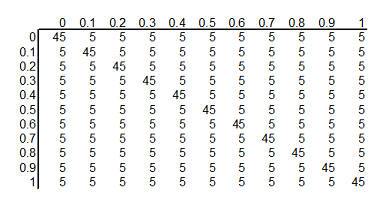
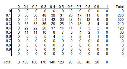
You can arrange these prior probabilities into a rectangular grid where the
columns represent a specific survival rate with ECMO and the rows represent a
specific survival rate with conventional therapy. To simplify the display, we
multiplied each probability by 1000 and rounded the result. So we have 121
hypotheses, ranging from ECMO and conventional therapy both having 0% survival
rates to ECMO having 100% survival and conventional therapy having 0% survival
rates to ECMO having 0% and conventional therapy having 100% survival rates to
both therapies having 100% surivival rates. Each hypothesis has a probability
assigned to it. The probability for ECMO 90% and conventional therapy 60% has a
probability of roughly 5 in a thousand and the probability for ECMO 80% and
conventional therapy 80% has a probability of roughly 45 in a thousand.
The second step in a Bayesian data analysis is to calculate P(E | H), the
probability of the observed data under each hypothesis. If the ECMO survival
rate is 90% and the conventional therapy survival rate is 60%, then the
probability of observed 28 out of 29 survivors in the ECMO group is 152 out of
one thousand, the probability of observing 6 out of 10 survivors in the
conventional therapy group is 251 out of one thousand. The product of those two
probabilities is 38,152 out of one million which we can round to 38 out of one
thousand. If you've forgotten how to calculate probabilities like this, that's
okay. It involves the binomial distribution, and there are functions in many
programs that will produce this calculation for you. In Microsoft Excel, for
example, you can use the following formula.
- binomdist(28,29,0.9,FALSE)*binomdist(6,10,0.6,FALSE)
The calculation under different hypotheses will lead to different
probabilities. If both ECMO and conventional therapy have a survival probability
of 0.8, Then the probability of 28 out of 29 for ECMO is 11 out of one thousand,
the probability of 6 out of 10 for conventional therapy is 88 out of one
thousand. The product of these two probabilities is 968 out of one million,
which we round to 1 out of one thousand.
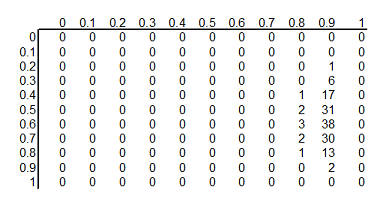
The table above shows the binomial probabilities under each of the 121
different hypotheses. Many of the probabilities are much smaller than one
out of one thousand. The likelihood of seeing 28 survivals out of 29 babies in
the ECMO survivals is very small when the hypothesized survival rate is 10%,
30%, or even 50%. Very small probabilities are represented by zeros.
Now multiply the prior probability of each hypothesis by the likelihood of
the data under each hypothesis. For ECMO=0.9, conventional therapy=0.6, this
product is 5 out of a thousand times 38 out of a thousand, which equals 190 out
of a million (actually it is 173 out of a million when you don't round the data
so much). For ECMO=conventional=0.8, the product is 45 out of a thousand times 1
out of a thousand, or 45 out of a million.

This table shows the product of the prior probabilities and the likelihoods.
We're almost done, but there is one catch. These numbers do not add up to 1
(they add up to 794 out of a million), so
we need to rescale them. We divide by P(E) which is defined in the wikipedia
article as
P(E) = P(E|H1) P(H1) + P(E|H2) P(H2) + ...
In the example shown here, this calculation is pretty easy: add up the 121
cells to get 794 out of a million and then divide each cell by that sum. For more complex setting, this
calculation requires some calculus, which should put some fear and dread into
most of you. It turns out that even experts in Calculus will find it
impossible to get an answer for some data analysis settings, so often Bayesian
data analysis requires computer simulations at this point.
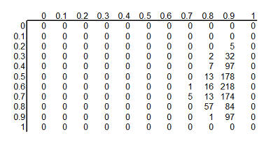
Here's the table after standardizing all the terms so they add up to 1.
This table is the posterior
probabilities, P(H | E). You can combine and manipulate these posterior
probabilities far more easily than classical statistics would allow. For example, how likely are we to believe the hypothesis that ECMO
and conventional therapy have the same survival rates? Just add the cells along
the diagonal (0+0+...+5+57+97+0) to get 159 out of a thousand. Prior to
collecting the data, we placed the probability that the two rates were equal at 500 out of a thousand, so the
data has greatly (but not completely) dissuaded us from this belief. You can
calculate the probability that ECMO is exactly 10% better than conventional
therapy (0+0+...+1+13+84+0 = 98 out of a thousand), that ECMO is exactly 20%
better (0+0+...+13+218+0 = 231 out of a thousand), exactly 30% better
(0+0+...+7+178+0 = 185 out of a thousand), and so forth.
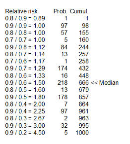
Here's something fun that Dr. Albert didn't show. You could take each of the
cells in the table, compute a ratio of survival rates and then calculate the
median of these ratios as 1.5 (see above for details). You might argue that 1.33
is a "better" median because 448 is closer to 500 than 666, and I wouldn't argue
too much with you about that choice.
Dr. Albert goes on to show an informative prior distribution. There is a fair
amount of data to indicate that the survival rate for the conventional therapy
is somewhere between 10% and 30%, but little or no data about the survival rates
under ECMO.
The table above shows this informative prior distribution. Recall that the
rows represent survival rates under conventional therapy. This prior
distribution restricts the probabilities for survival rates in the conventional
therapy to less than 70%. There is no such absolute restriction for ECMO, though
the probabilities for survival rates of 70% and higher are fairly small.
Repeat of pop quiz
Review the pop quiz presented earler. Do you feel more confident in your
answers?
What now?
Go to the main page of the P.Mean website
Get help
 This work is licensed under a
Creative
Commons Attribution 3.0 United States License. This page was written by
Steve Simon and was last modified on
2017-06-15.
This work is licensed under a
Creative
Commons Attribution 3.0 United States License. This page was written by
Steve Simon and was last modified on
2017-06-15.