P.Mean >> Statistics webinar >> The first three steps in data entry, with examples in PASW/SPSS (to be presented in November 2009).
This talk uses material from my old website
as well as some new material.
Content: This training class will give you a general introduction to data management using PASW (formerly known as SPSS) software. This class is useful for anyone who needs to enter or analyze research data. Students should know how to use a mouse and how to open applications within Microsoft Windows. No statistical experience is necessary. There are three steps that will help you get started with data entry for a research project. First, arrange your data in a rectangular format (one and only one number in each intersection of every row and column). Second, create a name for each column of data and provide documentation on this column such as units of measurement. Third, create codes for categorical data and for missing values. This class will show examples of data entry including the tricky issues associated with data entry of a two by two table and entry of dates.
Objectives: In this class, you will learn how to:
- document variables in a PASW data set;
- enter and manipulate dates in PASW; and
- import data into PASW from other programs.
Teaching strategies: Didactic lectures and individual computer exercises.
Outline:
- Spreadsheet or database
- General guide to data entry
- Importing spreadsheet data into SPSS
- Importing database files into SPSS
- Inputting a two-by-two table into SPSS
- Date calculations in SPSS
Spreadsheet or Database?
Dear Professor Mean, I am not sure whether I should use a database or a spreadsheet to enter my data?
For data entry, there are several advantages for a database. Databases easily allow you to implement quality checks. They also allow you to easily integrate data from multiple sources. Finally, they are more effective in handling very large data sets.
On the other hand, spreadsheets are faster to set up and allow easier copying and duplication for data with repetitive patterns. Before you choose, make sure that the statistical software can import data from your database or spreadsheet.
Advantages of a database
First, databases allow you to implement quality checks in the data. For example, one of your variables might be gender. It might be coded 1=Male, 2=Female, 9=Unknown (though if gender is unknown, you might want to look at the credentials of the doctor doing the examination). With a database, you could set up data entry in that field so that it would beep anytime you tried to enter something other than a 1, 2, or a 9.
Another quality check found in databases is insuring that the same id code is not assigned to two different subjects. Database specialists refer to this as checking for unique primary keys.
It's also possible to program a database to check for consistencies in dates. If the birth date is in 1994, for example, and the examination date is in 1987, then either your data are in error or you have an extremely far-sighted pre-natal care program.
Yet another example is checking the gender or age of the subject before allowing certain data to be entered. Male subjects, for example, would not normally have a hysterectomy in their medical history. Five year olds are rarely married or widowed. The range of quality checks you can include in a database is limited only by your imagination.
Second, a database is effective at integrating data coming from a variety of sources. For example, you might have data coming from a laboratory, a questionnaire, and from the medical records. A database makes it easy to properly link the information from all three sources.
Another example of where a database is extremely useful is in a multi-center clinical trial. The database offers a standard way for data entry that helps avoid the inconsistencies that can plague such studies.
Of course, if you have a data set so complex as to take information from three different sources, then you should definitely consult an expert early in the design of your study. Databases are nice, but they are no substitute for careful planning.
Third, a database is more effective at handling very large data sets. Unlike a spreadsheet, the entire data set does not have to fit into computer memory. Of course, this is a factor only when the data set on the order of tens of thousands of records or more. If your data set is smaller than this then fitting all of the data into computer memory is unlikely to be a problem.
Advantages of a spreadsheet
On the other hand, spreadsheets can be up and ready for data entry faster than databases. The extra time required by a database might be beneficial, but for a simple data entry situation, it might just as easily be overkill.
Spreadsheets also are more efficient at copying and duplicating blocks of information. This can be a time-saver for data sets with repetitive patterns, such as multi-factorial experiments.
Other considerations
Before you choose, check to make sure that the statistics software can import your version of the spreadsheet or database. SPSS for Windows, for example, can import Excel and Lotus spreadsheets, dBase format databases like FoxPro, as well as any database or spreadsheet which supports the ODBC (Open Data Base Connectivity) standard, like Access.
Before you make your choice, be sure to factor in any human considerations. If the person doing data entry is much more comfortable with a spreadsheet than a database (or vice versa), that might outweigh some of the computer efficiencies. On the other hand, keep in mind that software in general, and database software in particular, is getting easier to use. Don't let lack of experience keep you from trying a database. It's easier than you think.
Summary
In summary, databases allow for better error checking, for better integration of data from multiple sources, and for better handling of very large files. Spreadsheets are faster to get up and running, which can be an advantage for small tasks. Spreadsheets also have an advantage when there are repetitive patterns in the data.
Which to choose? It may come down to how large and complex your data set is. The bigger and messier the data, the more a database can help.
General guide to data entry.
Dear Professor Mean, I'm about to start typing in my research data. Do you have any general guidelines for data entry?
Every data set is different, but most data entry procedures will start out the same. Here are the first three steps that you should follow to help insure a successful data entry.
- Arrange your data in rectangular format.
- Create variable names (8 characters or less).
- Assign number codes for categorical data and missing values.
Here are more details about each guideline.
1. Arrange your data in rectangular format.
Arrange your data in a rectangular format. The intersection of each row and column should contain a single number. Don't leave a cell empty if you can possibly avoid it. Empty cells are ambiguous (does it represent a missing value or is it a sign that data entry is not yet complete on this patient). Some computer programs (not PASW) will take an empty cell and convert it to zero, which can lead to disastrous results. Suppose that a column of data represents the age of the mother at the birth of her first child. If an unknown age is converted to a zero age (the ultimate in babies having babies), then any statistics you compute on that column will be grossly distorted.
Sometimes it will take a bit of restructuring and rearrangement to create a rectangular grid (as in the example below), but the effort is usually worth it. A rectangular grid almost always lends itself more easily to data analysis.
The flip side of not leaving a cell empty is to never try to squeeze two numbers into the same cell. You might be tempted, for example, to list blood pressure as 120/80 to represent the systolic and diastolic pressures. Don't do this! You will make it difficult for the computer to compute an average blood pressure of any type. Furthermore, some computer software programs might look at the entry 120/80, misinterpret the slash as a division sign, and replace the whole cell with 1.5.
Here's an example of data which does not fit into a rectangular format. These data are loosely based on a study of breast feeding in pre-term infants. The data have been shortened and modified to serve as a simple example of data entry.
Breast feeding status at six months

No                   Yes                  Lost to follow-up

Mom's Marital Birth  Mom's Marital Birth  Mom's Marital Birth
Age   Status  Weight Age   Status  Weight Age   Status  Weight

 18   Married 1.550   28   Single  2.381   28   Married 1.685
 33   Single  1.990                1.130                2.435
 34   Married         26   Married 2.060
 36   Married 1.640
Notice the jagged shape of the data. There is a 4 by 3 block of data (the No group), and then a 3 by 3 block of data (the Yes group), and then a 2 by 3 block of data (the Lost to follow-up group). If we stack these blocks one beneath another rather than one beside another, we will get a rectangular shape. When we re-arrange the data, however, we need to include an extra column of information to designate the specific block/group.
Here is what the data looks like after we re-arrange it into a rectangular format.
Breast
Feeding  Mom's Marital Birth
Status   Age   Status  Weight

 No       18   Married 1.550
 No       33   Single  1.990
 No       34   Married
 No       36   Married 1.640
 Yes      28   Single  2.381
 Yes                   1.130
 Yes      26   Married 2.060
 Lost     28   Married 1.685
 Lost                  2.435
2. Assign codes for categorical data and missing values.
If you have categorical data, assign a code to each category level. Use the code during data entry to save time and minimize errors.
Here are some examples of codes: Gender 1=Male, 2=Female, 9=Unknown; Race 1=White, 2=Black, 3=Asian, 4=Hispanic, 5=Native American, 8=Multiracial, 9=Unknown; Likert scale 1=Strongly Disagree, 2=Disagree, 3=Neutral, 4=Agree, 5=Strongly Agree, 9=No answer.
While I prefer to use number codes, there are some advantages to using short letter codes. Here are some examples of letter codes: Gender M, F, and U (Male, Female, and Unknown); Race W, B, A, H, N, M, and U (White, Black, Asian-American, Hispanic, Native American, Mixed, and Unknown); Likert scale SD, D, N, A, SA, NA (Strongly Disagree, Disagree, Neutral, Agree, Strongly Agree, No Answer). Letter codes are easier to remember, and sometimes can be used effectively as plotting symbols.
For binary variables, I prefer to use 0-1 coding rather than 1-2. It is similar to how computers work (0=off, 1=on). I use 0 for example, for the control/placebo group and 1 for the control group.
I prefer number codes because they offer more flexibility during statistical analysis. For example, SPSS will not allow you to draw a scatterplot when one of your variables uses letter codes. Other software will alphabetize your letter codes, which may not be what you intended. For example, an alphabetized Likert scale would be printed in the following meaningless order:
- Agree,
- Disagree,
- Neutral,
- No Answer,
- Strongly Agree,
- Strongly Disagree.
Letter codes do have advantages. If you code a variable for sex as 1 and 2, it is easy to get confused about whether 1 is males and 2 is females or vice versia. Coding sex as M or F is not going to lead to such confusion.
Letter codes are certainly acceptable, but let's assign number codes for the categorical variables in the breast feeding data example. For br_feed, let 0=No, 1=Yes, and 9=Lost. For mar_st, let 0=Single; 1=Married, and 9=Missing. With this change, the data will look like this:
Breast
Feeding    Mom's  Marital    Birth
Status     Age    Status     Weight

   0        18       1       1.550
   0        33       0       1.990
   0        34       1
   0        36       1       1.640
   1        28       0       2.381
   1                         1.130
   1        26       1       2.060
            28       1       1.685
                             2.435
Whether you use number or letter codes, though, do make it a habit to document those codes. In PASW, that means defining value labels for each and every categorical variable (see below).
Note also that there are still some blank spots in this data. These represents missing data. Never let a empty field represent missing data. Explicitly create a code for missing, and be sure to explain why the data are missing to anyone involved with analysis of your data. In this example, let -1 represent a missing value for Mom's Age and Birth Weight. Let 9 represent a missing value for Marital Status.
Here's what the data looks like when we plug up the missing value holes.
Breast
Feeding    Mom's  Marital    Birth
Status     Age    Status     Weight

   0        18       1       1.550
   0        33       0       1.990
   0        34       1          -1
   0        36       1       1.640
   1        28       0       2.381
   1        -1       9       1.130
   1        26       1       2.060
   9        28       1       1.685
   9        -1       9       2.435
3. Create a name for each column of data and provide additional documentation such as units of measurement.
If you are using a spreadsheet, place a descriptive variable name at the top of each column. If you are using a database, provide a descriptive name for each field. You will use this variable or field name in statistical software like SPSS to specify the variables that you want to analyze. Try to be reasonably descriptive with your variable names; avoid generic names like VAR01, VAR02, etc.
While a spreadsheet or a database generally places few restrictions on variable names, most statistical software (including SPSS) will not be able to handle long names or names with special symbols. Here are some general guidelines that will help avoid trouble.
Use a brief name (eight to sixteen characters long). A long time ago, (version 11 and earlier of SPSS), you could not use a name longer than eight charcter long. Now you can use up to 255 characters, but you should show some restraint. You can add extra information in the variable label, if you like, but it is convenient to have a short "handle" that you can refer to for any column of data in your data set.
A mixture of numbers and letters is okay, but avoid special symbols such as $, &, or %. Most statistical software will reserve these special symbols for other purposes. The one major exception is the underscore (_), which is found usually paired on the same key with the minus sign. In fact, when SPSS imports names with special characters, it replaces them with the underscore character.
Don't rely on upper/lower case to distinguish among variable names (for example, don't name one variable x and the next one X). Some packages are case insensitive and even if they are not, having two variables with names that look almost identical is a formula for trouble.
Avoid embedded blanks. In most statistical software, an embedded blank will cause the software to presume that you are referring to two variables. If you are stringing together two or three words to represent a variable name (mom age or breast feeding status), just placing them next to one another can cause confusion (momage looks like a nonsense word rhyming with homage). There's a story about a website for a group known as Writer's Exchange. They used the URL: www.writersexchage.com, but someone noticed that this could be read as writer sex change. If your variable name consists of two or three short words, here are three strategies that work well.
- Use an upper case letter at the start of each new word: MomAge, BreastFeedingStatus.
- Separate words using a period: mom.age, breast.feeding.status
- Separate words using an underscore mom_age, breast_feeding_status.
Note that separating using a dash (minus sign) is not a good idea. A variable with the name mom-age looks too much to some computers like a subtraction calculation. Some software programs also use a dash to indicate a range of variables (a1-a8).
Here's what the data set looks like with variable names.
br_feed  mom_age  mar_st   birth_wt
   0        18       1       1.550
   0        33       0       1.990
   0        34       1          -1
   0        36       1       1.640
   1        28       0       2.381
   1        -1       9       1.130
   1        26       1       2.060
   9        28       1       1.685
   9        -1       9       2.435
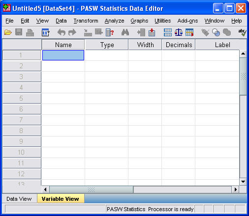
Once you have names for each column of data, you should document what goes into each column, and control how it is displayed. In PASW, there are several steps. It starts with selecting the VARIABLE VIEW tab to add documentation to your data.
From VARIABLE VIEW tab, you can tell SPSS how to display the data in the SPSS data editor window (how many decimal places shown, how dates are displayed, and how wide the columns are). You can also provide SPSS with informational labels that will appear in your output window (labels for the variable itself and, if needed, labels for category levels). You would also use the dialog box to specify any codes that represent missing data.
More details
There are a lot of important ways in which you can document your data. Start with the variable name itself, a brief description of up to eight characters of what this column of data contains. Then specify the format type (numeric, string, or date) for the data that is in this column. Now you can provide a longer description of your variable in the variable label. If your data are categorical, you can describe those categories using values labels. Finally, make sure that SPSS know which code, if any, you use to designate missing values. Repeat this task for each column of data.
Variable name
When documenting your data, your first step should be to provide a brief but descriptive variable name. This goes into the NAME column of the VARIABLE VIEW tab. SPSS provides a default of VAR00001 for the first column, VAR00002 for the second column and so forth. This coding is convenient in that it allows you to produce names for up to 99,999 columns of data. But if you have that much data, I hope you will get some help with your data entry.
Please spend some time to provide descriptive variable names. As noted above, these names should be short (8 to 16 characters). You will get a chance to provide additional details in the LABEL field.
After you provide a variable name, take a look at the other columns in the VARIABLE VIEW tab. Of special interest are the following:
- TYPE
- WIDTH
- DECIMALS
- LABELS
- VALUES
- MISSING
Format type
Click in the TYPE column to add or change the format type. You will notice a gray button appear on the right hand side. Click on it to get VARIABLE TYPE dialog box.
This dialog box has information about the type of data that you want to use. The most common data type is NUMERIC, which is used for any data that can be represented solely by numbers. If you have numeric data, you should tell SPSS the width of your numbers and how many decimal places you want displayed. Unless you are dealing with unusually large numbers, the default width of 8 works well. For some situations, you might be tempted to use a smaller makes, but this can make it more difficult to view the variable name and the value labels.
Be sure to set the number of decimal places appropriately. Please do not display decimal places that you don't really need. When you are looking at a list of numbers with values like 1.00, 2.00, 3.00, 4.00, it is much harder to read than the simpler 1, 2, 3, 4. Easy to read means easier to spot errors, so this is not a trivial issue.
For data with number codes or count data, you should change the number of decimal places to zero from the default of two. It's a minor point, but the superfluous .00 at the end of every number will make your data harder to read. For some data, you may instead need to display more than two decimal places. Keep in mind, though, that this dialog box controls how the data are displayed in the data editor window and not (for the most part) how they are displayed in the output window.
Select the STRING options for data that is all letters or a mixture of letters and numbers. When you select this option, SPSS provides a chance for you to tell how long the strings are.
If you click on the DATE option, you will be given choices between various display formats (month names versus month numbers, two digit versus four digit years, etc.). After all the publicity about the year 2000 problem, I don't need to lecture you on being careful with dates. But also remember that people disagree over whether the month or the date should appear first. Both Europe and the United States agree that 1/1/2009 is the first day of the year, but in Europe the last day is 31/12/2009 compared to 12/31/2009 in the United States.
Variable and value labels
Click on the label field to add a variable label. A variable label is a longer description of your data. Variable labels appear in your output and make it easier to follow what is going on. You can use a mixture of upper and lower case here, which I recommend for improving readability. AVOID USING ALL UPPERCASE HERE BECAUSE IT IS FAR LESS READABLE THAN A MIXTURE OF CASES.
You can put blanks and special symbols in your variable label. If you are very excited about a variable, spice it up with a couple of exclamation points. Go ahead and type to your heart's content. Just a small warning though. A variable label that is too long can make your output look a bit unwieldy. Although you can type up to 255 characters here, it looks strange to have a six inch label underneath a two inch histogram. A variable label of around 20 to 40 characters in length works well in practice.
You can also specify value labels in this dialog box. Value labels provide informative names for levels in any categorical variable. Leave the value labels blank for continuous data like weight or height. They do make sense, though, for categorical data like gender. This will serve as a reminder that data values of 1 represents males and 2 females. The last thing you want is for people to think that you can't tell the difference between males and females.
Value labels have to be defined one by one. Type in the number (or letter) code for your category in VALUE field, the value label in the VALUE LABEL field just beneath it and then click on the ADD button. Repeat this for your second category level and so forth.
Missing value codes
If needed, click on the MISSING VALUES button to designate missing value codes. Missing value codes are useful for designating data in SPSS where the value is unknown, not applicable or otherwise not provided.
Be careful about missing values. Values can be missing because the subject dropped out of the study. Perhaps you are looking for chemical concentrations that are sometimes too low for a laboratory to detect. Perhaps a subject refused to respond to a certain question. Perhaps you are asking for something like a spouse's age that is not applicable for a single person. Make sure you understand why your data is missing and discuss this issue with anyone you are consulting with. The statistical handling of missing values can vary greatly depending on how the value came to be missing.
When you are planning your project, it is a good idea to select a very clearly impossible code for your missing value. For example, use -1 for a birth weight because any infant with a negative birth weight would float up to the ceiling after delivery. Use a value of 9 to code missing for gender, since it is obvious to most of us that the number of possible genders is much smaller than 9.
Column format
I usually ignore the COLUMN FORMAT button, but you can click here if you like. If you didn't specify a width that differs from the SPSS default width of 8 earlier, you can do so here. You can also tell SPSS to left justify, center, or right justify this column of data in the data editor window. SPSS chooses a logical default of left justification for strings and right justification for just about everything else.
Example
Let's see how to document a column of data that represents marital status. Marital status is a categorical variable with five codes (1=single, 2=married, 3=divorced, 4=widowed, 9=unknown). I know this is slightly different than the example above, but I wanted to show an example of a categorical variable with many value.
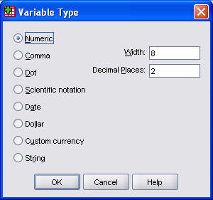
We use numeric codes for this variable, so we keep the NUMERIC option selected. With no values larger than 9, we could change the WIDTH field a little bit, but anything much smaller than 8 makes it difficult to see the variable name and the value labels later. The number codes here do not require any decimals, so we change the DECIMAL PLACES field from 2 to 0.
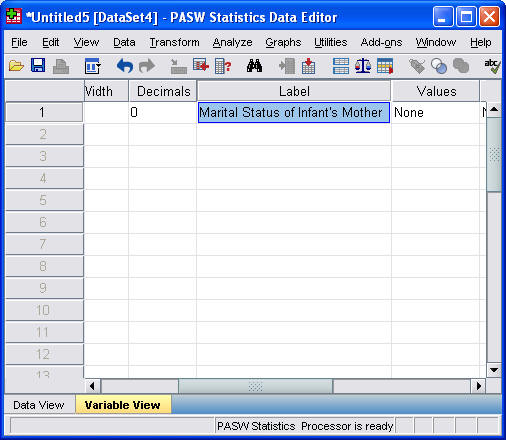
A nice variable label is "Marital Status of the Infant's Mother". Notice that we can include an apostrophe here. I also used a mixture of upper and lower case. This is easier to read than all lower case and much easier than all upper case.
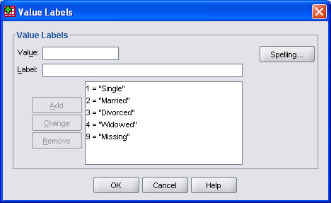
The value labels are "Single"; "Married"; "Divorced"; "Widowed"; and "Unknown". Notice again that I use mixed case. Value labels are appropriate here because this is a categorical variable. For a continuous variable like birth weight, we would leave the value labels blank.
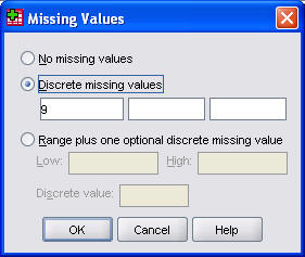
Finally, I designate 9 as a missing value.
Summary
To get started with data entry, follow these three steps.
- Arrange your data in rectangular format.
- Create codes for category levels and missing values.
- Create variable names (8 characters or less).
Follow these steps before entering your data and you will simplify the process of importing your data into a statistical software package like PASW.
Importing spreadsheet data into SPSS.
Dear Professor Mean, I need to import data in an Excel spreadsheet, but I can't get SPSS to read this data properly. Can you help? -- Stumped Stan
Dear Stumped, You probably didn't hear, but SPSS changed its name with version 17 to PASW. I like to think of it as the software formerly known as SPSS.
One obvious warning. You can't import data from Excel into PASW while the file is still open in Excel. Excel places an electronic lock on the file when it is open so that you can't have the same spreadsheet open twice. PASW notices this lock and backs away thinking that something is wrong. It's actually a good thing because if you have unsaved changes in Excel and you import the file before those changes are saved, you will have invalid data in PASW.
You should also do some prep work before you import Excel data. Excel is an extremely flexible program that allows you to put your data in just about any way you like.
Here are the first three steps that I recommend for manipulating Excel data prior to import into PASW.
- Arrange the data in a rectangular grid
- Don't mix strings and numbers in a single column.
- Put descriptive names in your first row.
Rectangular grid
A rectangular gird is a systematic layout of your data so that that the intersection of every column and row contains a single number. The data should start in the first row of the spreadsheet, or the second row, if you use the first row as column labels. Don't leave any "holes" in the spreadsheet.
Be sure to delete any rows of your spreadsheet that contains summary data like totals or means. You don't want SPSS to think that this summary row is just another row of data. Charts will probably be ignored, but it wouldn't hurt to remove those also.
After you import your data, you may notice a bunch of blank columns to the right or a bunch of blank rows at the bottom. These appear unpredictably, but I think they relate to the print range that was set in Excel. Possibly it represents an extension to a cell that was formatted a long time ago, but no data was entered. If you see these blank columns or rows, be sure to delete them. They don't hurt anything, but they are annoying.
Don't mix strings and numbers.
A mixture of strings and numbers in a single column will confuse SPSS. SPSS uses the first value that it sees in a column to decide if that column should be stored using string, date, or numeric format. If any further values in that column do not match the format of your first value, SPSS will convert that value to missing.
Here's an example of a mixture of strings and numbers "1", "2", "3 or more". This type of coding will ensure that a large amount of your data gets converted to missing values. Which values stay and which ones don't depend on what appears first in your column.
Provide brief descriptive names
SPSS can use the first row of your spreadsheet as variable names, as long as you keep within the proper restrictions. Keep you names short. Although the previous restriction to eight characters or less, names that are very long become unwieldy and don't display well in the graphs and tables. You can (and should) use the variable label in SPSS to provide a longer and more detailed description of this variable.
The name has to be one word with no blanks. You can use the underscore symbol "_" or the dot to simulate blanks. You can also use MixedCapitalization to simulate blanks.
Avoid special symbols (other than the underscore and dot). Symbols like the dash (-) and the slash (/) cause problems because they imply some sort of arithmetic operation.
A variable name like "Mother's Age" causes problems because it includes a special symbol (the apostrophe) and it has a blank. If you tried to use this name, SPSS would create a generic name like VAR00001 and use "Mother's Age" as a variable label. A name that SPSS will tolerate would be "mom_age" or "MomAge" or "mom.age".
It takes some creativity to describe a variable well with only eight characters. Do the best you can. Remember that you can always add a lengthy variable label later that has blanks, special symbols.
Example
Here is an Excel spreadsheet with data from a house pricing study. I have already arranged the data in a rectangular grid and placed brief descriptive names in the first row..
Open SPSS and select FILE | OPEN from the menu. Here is the SPSS dialog box that you will see. Click on the down arrow in the FILE OF TYPE field and select the EXCEL (*.XLS) option. Find your file on the proper drive and folder of your computer.
When you click on the OPEN button, you get the dialog box shown below. Click on the READ VARIABLE NAMES BUTTON if the first row of your spreadsheet has variable names. Then click on the OK button.
Check if you got the correct number of variables (columns) and cases (rows). A common problem is that SPSS will sometimes import a bunch of extra blank rows. You can delete these manually.
Here is what the SPSS data window looks like. You are now ready to do things like adjusting the number of decimal places displayed and adding documentation (see above for details).
Summary
If you want to import Microsoft Excel data into SPSS, follow these four steps:
- Close the Excel file
- Arrange the data in a rectangular grid
- Don't mix strings and numbers.
- Put descriptive names in your first row.
Once you have done this, select FILE | OPEN DATA from the SPSS menu. Then click on FILE OF TYPE field and select the EXCEL (*.XLS) option.
This webpage was written by Steve Simon on 1999-08-20, edited by Steve Simon, and was last modified on 2008-07-08. Send feedback to ssimon at cmh dot edu or click on the email link at the top of the page. Category: Ask Professor Mean, Category: Data management, Category: SPSS software
Importing database files into SPSS.
Dear Professor Mean, How do I import database files into SPSS? I don't want to re-type everything, because there are 70,000 records. The data are stored in a Microsoft Access file. -- Vexed Vidya
Dear Vexed, SPSS can import data from a variety of sources using a system known as ODBC (Object Data Base Connectivity). ODBC has links to just about every database that you would ever need to use.
Short explanation
I'll show you an example using Microsoft Access, but this would work just as well on other database systems, such as Oracle and Informix. To import data from Access, select FILE | DATABASE CAPTURE | NEW QUERY from the SPSS menu.
More details
When you import data using ODBC, SPSS asks you what type of data source you want to import from. On my system, I have the ability to import Access, Excel, and FoxPro files. Through Microsoft Windows, I can add the capability of importing from other sources like Oracle or Informix if I needed these formats.
I can also specify a particular location that I want to import from on a repeated basis. In the example I show later, you will see that I have defined data sources labelled "ghstudy", Menninger", "patient complaints", "Santos" and "x". Providing a pre-specified location for my import is especially useful for databases that are being updated on a regular basis. If you want to define such a source, you can click on the ADD DATA SOURCE button, but I will not provide any details about it in this handout.
After you specify the type of data you want to import, SPSS will ask you for the following details.
- Where the data are located
- The table or tables in your database you want to import
You also have the following options
- Specifying relationships between tables
- Selecting a subset of your data
- Renaming some of the variables
- Saving the query for re-use
Saving the query for re-use is another way of simplifying repeated imports from the same data set. Saving the query will save not only the location of hte database you want to import from, but also the information about subsets, changes in variable names, etc.
Example
Here is an example of importing an Access database with data from a growth hormone study. Select FILE | DATABASE CAPTURE | NEW QUERY from the SPSS menu FILE | DATABASE CAPTURE | NEW QUERY from the SPSS menu.
The dialog box shown above allows you to select your data source. Click on ACCESS 97 and then click on the NEXT button.
The dialog box shown above asks you for a location for your Access database. Be sure that you select the correct drive and folder. Then click on the file, and click on the OK button.
SPSS gives you a list of all available tables and queries within this database.
The dialog box shown above gives you a list of all available tables and queries within this database. Drag the table from the AVAILABLE TABLES field into the RETRIEVE FIELDS IN THIS ORDER field. If you want data from more than one table/query, repeat this process. If there are some variables you do not want to import, drag them out of the RETREIVE FIELDS IN THIS ORDER field.
If you have a simple import, you can click on the FINISH button now. If you click on the NEXT button instead, SPSS will give you some options to fine tune your import. You can
- Specifying relationships between tables
- Selecting a subset of your data
- Renaming some of the variables
- Saving the query for re-use
Saving the query for re-use is another way of simplifying repeated imports from the same data set. Saving the query will save not only the location of the database you want to import from, but also the information about subsets, changes in variable names, etc.
Inputting a two-by-two table into SPSS.
Dear Professor Mean, I have the following data in a two by two table:
| D+ | D- | Total | |
| F+ | 34 | 23 | 57 |
| F- | 139 | 119 | 258 |
| Total | 173 | 142 | 315 |
When I try to enter this data into SPSS, I can't get it to compute risk ratios and confidence intervals. What am I doing wrong? -- Jinxed Jason
Dear Jinxed, You have values ranging from F- to D+? I hope this isn't data on the grades you received in college.
Actually these data are from a paper: Sands et al (1999). F+ represents presence of a risk factor (in this case, previous miscarriage) and F- represents absence of that risk factor. D+ represents presence of a defect (ventricular septal defect or VSD) and D- represents absence of that defect.
Risk
FactorGroup Number/Total
(Percent)Odds Ratio
(95%CI)Miscarriage VSD
Control34/173 (20%)
23/142 (16%)1.3 (0.7,2.3) Female VSD
Control84/173 (49%)
60/142 (42%)2.1 (1.3,3.2) Low parity VSD
Control76/173 (44%)
58/142 (41%)1.1 (0.7,1.8) Smoking VSD
Control41/173 (24%)
39/139 (28%)0.8 (0.5,1.3) Alcohol VSD
Control18/173 (10%)
20/139 (14%)0.7 (0.4,1.5) Notice that we have to do a bit of arithmetic to get all the values. If 34 out of 173 VSD cases had a previous miscarriage, then 139=173-34 did not. If 23 out of 142 controls had previous miscarriage as a risk factor, then 119 did not.
For data like this, you have to re-arrange things and then apply weights. The following discussion talks about SPSS, but the general method works for most other statistical software.
To re-arrange the data, you need to specify three variables: F, D, and COUNT. F takes the value of 1 for F+ and 0 for F-. D takes the value of 1 for D+ and 0 for D-. The 0-1 coding has some nice mathematical properties, but you could use 1 and 2 instead. For each combination of F and D we will record the sample size in COUNT.
Here's what your re-arranged data would look like
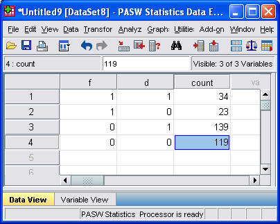
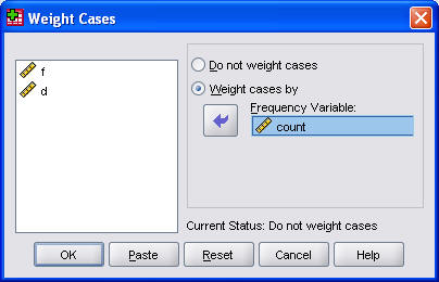
Enter the data, and tell SPSS that W represents a weighting variable, and you're ready to rock and roll. You do this by selecting Data | Weight Cases from the SPSS menu.
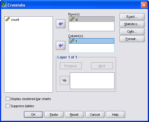
Then select Analyze | Descriptive Statistics | Crosstabs from the SPSS menu to create a two by two table.
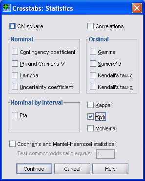
Be sure to click on the Statistics button and select the Risk option box to ask SPSS to compute the risk ratios.
I also usually find it useful to display the row percentages. To do this, click on the Cells button.
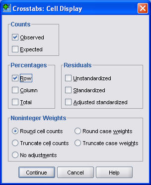
In the Crosstabs: Cell Display dialog box, select the Row Percentages option box. Here's what the first part of the output looks like.
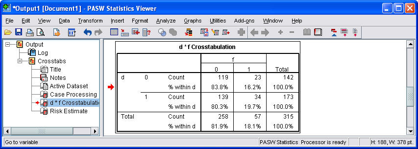
Notice that the rows and columns are reversed in this table. There are several ways to change how the table is displayed, but it is showing essentially the same information in any order.
Here is what the second part of the output looks like.
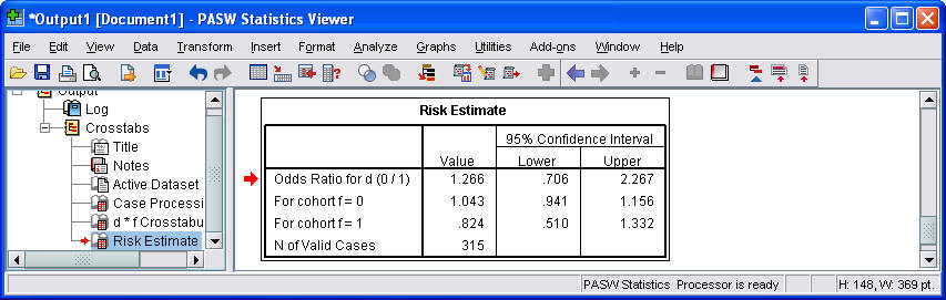
By the way, if you tried to use the crosstabs procedure without weighting, you would get exactly one observation in each cell. Pretty boring, eh?
Summary
Jinxed Jason can't figure out how to enter data from a two by two table into SPSS. Professor Mean explains that you need three variables to represent a two by two table. The first variable indicates the specific column of your table and the second variable indicates the specific row (or vice versa). The third variable indicates the count or frequency for each intersection of row and column. You do not include the row or column totals in your data entry. You can then select Analyze | Descriptive Statistics | Crosstabs from the SPSS menu to analyze the data from your two by two table. You get additional analyses by selecting the Risk and/or Chi-square option boxes.
Further reading
This webpage was written by Steve Simon on 1999-08-18, edited by Steve Simon, and was last modified on 2008-07-14. Send feedback to ssimon at cmh dot edu or click on the email link at the top of the page. Category: Ask Professor Mean, Category: Data management, Category: SPSS software
Date calculations in SPSS.
Dear Professor Mean, I am trying to use dates in SPSS for certain calculations. For example, I want to use a compute statement in SPSS to create a new variable called duration of injury (durinj). I know that I must subtract the date of injury from the date of interview. However, when I do this, I get a number in the millions. What am I doing wrong? -- Stumped Sharon
Dear Stumped, Maybe your patients were waiting for their HMO to approve a visit to a specialist.
Short explanation
SPSS stores date/time values as the number of seconds since October 14, 1582 (the start of the Gregorian calendar). If you specify only a date and not a time, then SPSS sets the time to midnight. When you subtract two dates, you get the duration of injury in seconds. Divide by 86,400 (=24*60*60) to get the duration of injury in days. Divide again by 7, 30, or 365.25 to get duration in weeks, months, or years.
More details
To see what SPSS is doing, reformat the date as a number. You will see something with a whole lot of digits. The date of 1/1/2000, for example, the date when all the antiquated software in the world will crash, is just a little more than 13 billion seconds to SPSS. Fortunately, SPSS allocates more than two digits here.
To subtract one column of numbers from another in SPSS, you select TRANSFORM | COMPUTE from the menu. Tell SPSS what name you want for this difference in the TARGET VARIABLE field. Then select the first variable and add it to the NUMERIC EXPRESSION field. Type in a minus sign (or click on the minus button in the mini calculator). Finally, select the second variable and add it to the NUMERIC EXPRESSION field after the minus sign.
If you are using dates, then this time interval is expressed in seconds. Place parentheses around the entire expression. Then place a slash at the end, followed by 86400. Dividing by 86400 changes the units from seconds to days.
Example
A common example using dates is computing length of stay in the hospital.
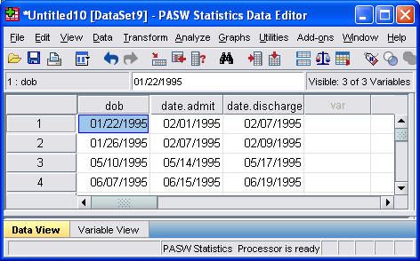
The data shown above represents the birthdate (dob), date of admission to the hospital (dateadm), and date of discharge from the hospital (datedsc) for newobrn babies admitted with a diagnosis of dehydration. To compute length of stay, you need to select TRANSFORM | COMPUTE from the SPSS menu.
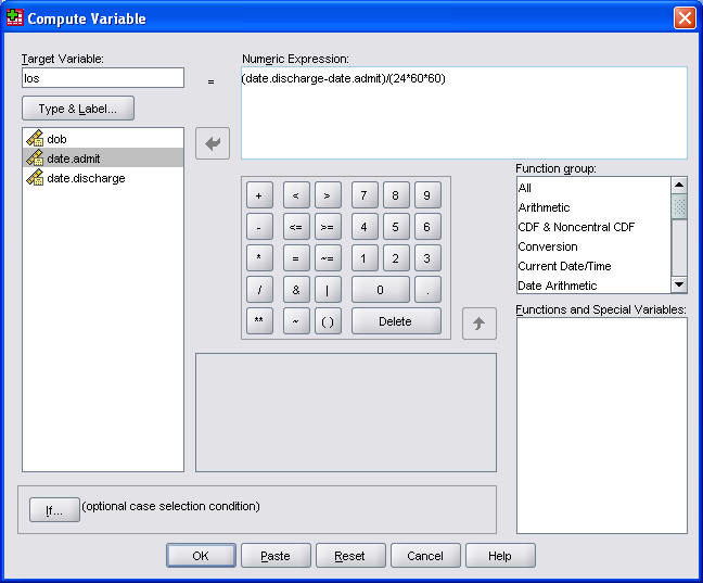
The figure shown above is the dialog box that you get. Type in a new name in the TARGET VARIABLE field. The formula for computing length of stay is
(datedsc-dateadm)/(24*60*60)which you should type into the NUMERIC EXPRESSION field. Then click on the OK button.
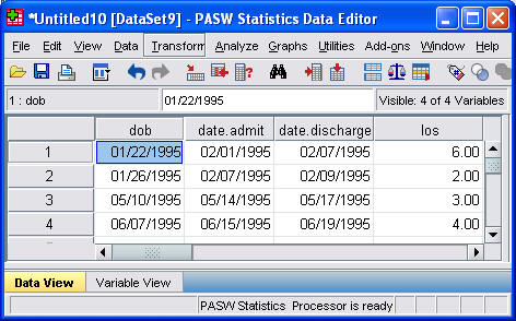
This figure shown above indicates that you have successfully computed length of stay as the difference between two date values. Congratulations.
Summary
Stumped Sharon is having problems with some calculations using dates in SPSS. Professor Mean explains that SPSS stores data values as the number of seconds since October 14, 1582. So when you calculate the difference between two date values, you see the number of seconds between the two events. Divide this difference by 86,400 (=24 hours * 60 minutes * 60 seconds) to re-express this as days.
Further reading
Raynald Levesque has a nice web tutorial about dates in SPSS.
- Dates Tutorial. Raynald Levesque. Accessed September 7, 2001.
http://pages.infinit.net/rlevesqu/LearningSyntax.htm#DateTutorial
Update
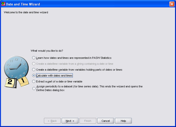
I attended a web seminar on the new enhancements in version 13.0 of SPSS software. The most notable change is in date calculations.
Date and time variables in SPSS have always been difficult. I have a web page showing some of the issues involved with computing the difference between two dates. SPSS has now added a Data and Time Wizard. Select TRANSFORM | DATE/TIME from the menu. Here's the first dialog box from that menu.
This is a very pleasant surprise, since dates are a source of constant confusion for me and for the people I work with. There were other enhancements, but to me this is the only important one.
What now?
![]() This work is licensed under a
Creative
Commons Attribution 3.0 United States License. This page was written by
Steve Simon and was last modified on
2017-06-15.
This work is licensed under a
Creative
Commons Attribution 3.0 United States License. This page was written by
Steve Simon and was last modified on
2017-06-15.