P.Mean >> Statistics webinar >> The first three steps in a logistic regression analysis, with examples in PASW/SPSS (to be presented in November 2009).
This talk uses material from my old website
as well as some new material.
You will use two SPSS data sets for practice exercises: bf.sav, and housing.sav. If you have trouble downloading these files, try
Outline:
- Description of the breast feeding data set
- Titanic mortality data set
- Definition: Categorical data
- Definition: Continuous data
- Inputting a two-by-two table into SPSS
- Definition: Odds
- Odds ratio versus relative risk
- The concepts behind the logistic regression model
- Overfitting the data
- Guidelines for logistic regression models
- SPSS dialog boxes for logistic regression
- Please fill out an evaluation form
Description of the breast feeding data set.
The file bf.sav contains data from a research study done at Children's Mercy Hospital and St. Luke's Medical Center. The data comes from a study of breast feeding in pre-term infants. Infants were randomized into either a treatment group (NG tube) or a control group (Bottle). Infants in the NG tube group were fed in the hospital via their nasogastral tube when the mother was not available for breast feeding. Infants in the bottle group received bottles when the mothers were not available. Both groups were monitored for six months after discharge from the hospital.
Variable list
- MomID Mother's Medical Record Number
- BabyID Baby's Medical Record Number
- FeedTyp Feeding type (Bottle or NG Tube)
- BfDisch Breastfeeding status at hospital discharge (Excl, Part, None)
- BfDay3 Breastfeeding status three days after discharge (Excl, Part, None)
- BfWk6 Breastfeeding status six weeks after discharge (Excl, Part, None)
- BfMo3 Breastfeeding status three months after discharge (Excl, Part, None)
- BfMo6 Breastfeeding status six months after discharge (Excl, Part, None)
- Sepsis Diagnosis of sepsis (Yes or No)
- DelType Type of delivery (Vag or C/S)
- MarStat Marital status of mother (Single or Married)
- Race Mother's race (White or Black)
- Smoker Smoking by mother during pregnancy (Yes or No)
- BfDurWk Breastfeeding duration in weeks
- AB Total number of apnea and bradycardia incidents
- AgeYrs Mother's age in years
- Grav Gravidity or number of pregnancies
- Para Parity or number of live births
- MiHosp Miles from the mother's home to the hospital
- DaysNG Number of days on the NG tube.
- TotBott Total number of bottles of formula given while in the hospital
- BirthWt Birthweight in kg
- GestAge Estimated gestational age in weeks
- Apgar1 Apgar score at one minute
- Apgar5 Apgar score at five minutes
Note: as I revise and improve this data set, I may add or remove variables from this list. So if the variables shown above don't match perfectly with the data set you have, don't panic.
Also note that I use different notation ("treatment" instead of "ng tube" and "control" instead of "bottle") in other parts of this website.
Source
Kliethermes PA; Cross ML; Lanese MG; Johnson KM; Simon SD [1999]. Transitioning preterm infants with nasogastric tube supplementation: increased likelihood of breastfeeding. J Obstet Gynecol Neonatal Nurs 28(3): 264-273
Description of the Titanic data set.
The file titanic.sav (also available as a text file) shows information about mortality for the 1,313 passengers of the Titanic. This data set comes courtesy of OzDASL and the Encyclopedia Titanica.
Variable list (5 variables)
There are several ways to categorize age, and I may include some of these in a future version of the data set.
Source:
OzDASL: Passengers on the Titanic. Smyth G. Accessed on 2002-12-13. "The data give the survival status of passengers on the Titanic, together with their names, age, sex and passenger class."
What is categorical data?
Data that consist of only small number of values, each corresponding to a specific category value or label. Ask yourself whether you can state out loud all the possible values of your data without taking a breath. If you can, you have a pretty good indication that your data are categorical. In a recently published study of breast feeding in pre-term infants, there are a variety of categorical variables:
Breast feeding status (exclusive, partial, and none);
whether the mother was employed (yes, no); and
the mother's marital status (single, married, divorced, widowed).
This webpage was written by Steve Simon on 2002-10-11, edited by Steve Simon, and was last modified on 2008-07-08.
What is continuous data?
Data that consist of a large number of values, with no particular category label attached to any particular data value. Ask yourself if your data can conceptually take on any value inside some interval. If it can, you have a good indication that your data are continuous. In a recently published study of breast feeding in pre-term infants, there are a variety of continuous variables:
This webpage was written by Steve Simon on 2002-10-11, edited by Steve Simon, and was last modified on 2008-07-08.
Inputting a two-by-two table into SPSS.
Dear Professor Mean, I have the following data in a two by two table:
| D+ | D- | Total | |
| F+ | 34 | 23 | 57 |
| F- | 139 | 119 | 258 |
| Total | 173 | 142 | 315 |
When I try to enter this data into SPSS, I can't get it to compute risk ratios and confidence intervals. What am I doing wrong? -- Jinxed Jason
Dear Jinxed,
You have values ranging from F- to D+? I hope this isn't data on the grades you received in college.
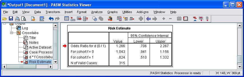
Actually these data are from a paper: Sands et al (1999). F+ represents presence of a risk factor (in this case, previous miscarriage) and F- represents absence of that risk factor. D+ represents presence of a defect (ventricular septal defect or VSD) and D- represents absence of that defect.
Risk
FactorGroup Number/Total
(Percent)Odds Ratio
(95%CI)Miscarriage VSD
Control34/173 (20%)
23/142 (16%)1.3 (0.7,2.3) Female VSD
Control84/173 (49%)
60/142 (42%)2.1 (1.3,3.2) Low parity VSD
Control76/173 (44%)
58/142 (41%)1.1 (0.7,1.8) Smoking VSD
Control41/173 (24%)
39/139 (28%)0.8 (0.5,1.3) Alcohol VSD
Control18/173 (10%)
20/139 (14%)0.7 (0.4,1.5) Notice that we have to do a bit of arithmetic to get all the values. If 34 out of 173 VSD cases had a previous miscarriage, then 139=173-34 did not. If 23 out of 142 controls had previous miscarriage as a risk factor, then 119 did not.
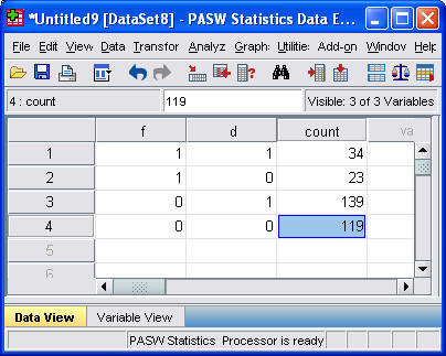
For data like this, you have to re-arrange things and then apply weights. The following discussion talks about SPSS, but the general method works for most other statistical software.
To re-arrange the data, you need to specify three variables: F, D, and COUNT. F takes the value of 1 for F+ and 0 for F-. D takes the value of 1 for D+ and 0 for D-. The 0-1 coding has some nice mathematical properties, but you could use 1 and 2 instead. For each combination of F and D we will record the sample size in COUNT.
Here's what your re-arranged data would look like
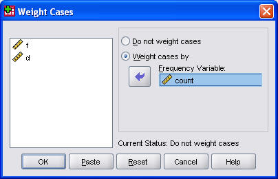
Enter the data, and tell SPSS that W represents a weighting variable, and you're ready to rock and roll. You do this by selecting Data | Weight Cases from the SPSS menu.
Then select Analyze | Descriptive Statistics | Crosstabs from the SPSS menu to create a two by two table.
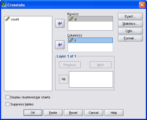
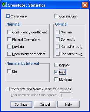
Be sure to click on the Statistics button and select the Risk option box to ask SPSS to compute the risk ratios.
I also usually find it useful to display the row percentages. To do this, click on the Cells button.
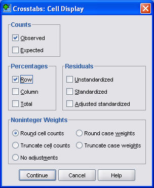
In the Crosstabs: Cell Display dialog box, select the Row Percentages option box.
Here's what the first part of the output looks like.
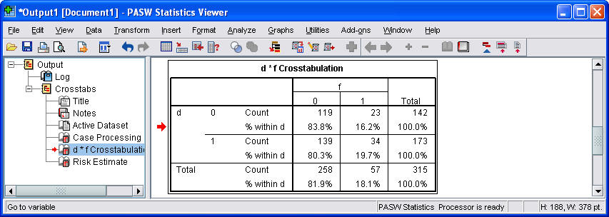
Notice that the rows and columns are reversed in this table. There are several ways to change how the table is displayed, but it is showing essentially the same information in any order.
Here is what the second part of the output looks like.
By the way, if you tried to use the crosstabs procedure without weighting, you would get exactly one observation in each cell. Pretty boring, eh?
Summary
Jinxed Jason can't figure out how to enter data from a two by two table into SPSS. Professor Mean explains that you need three variables to represent a two by two table. The first variable indicates the specific column of your table and the second variable indicates the specific row (or vice versa). The third variable indicates the count or frequency for each intersection of row and column. You do not include the row or column totals in your data entry. You can then select Analyze | Descriptive Statistics | Crosstabs from the SPSS menu to analyze the data from your two by two table. You get additional analyses by selecting the Risk and/or Chi-square option boxes.
Further reading
This webpage was written by Steve Simon on 1999-08-18, edited by Steve Simon, and was last modified on 2008-07-14.
What are odds?
The experts on this issue live just south of here in a town called Peculiar, Missouri. The sign just outside city limits reads "Welcome to Peculiar, where the odds are with you."
Odds are just an alternative way of expressing the likelihood of an event such as catching the flu. Probability is the expected number of flu patients divided by the total number of patients. Odds would be the expected number of flu patients divided by the expected number of non-flu patients.
During the flu season, you might see ten patients in a day. One would have the flu and the other nine would have something else. So the probability of the flu in your patient pool would be one out of ten. The odds would be one to nine.
More details
It's easy to convert a probability into an odds. Simply take the probability and divide it by one minus the probability. Here's a formula.
If you know the odds in favor of an event, the probability is just the odds divided by one plus the odds. Here's a formula.
You should get comfortable with converting probabilities to odds and vice versa. Both are useful depending on the situation.
Example
If both of your parents have an Aa genotype, the probability that you will have an AA genotype is .25. The odds would be
which can also be expressed as one to three. If both of your parents are Aa, then the probability that you will be Aa is .50. In this case, the odds would be
We will sometimes refer to this as even odds or one to one odds.
When the probability of an event is larger than 50%, then the odds will be larger than 1. When both of your parents are Aa, the probability that you will have at least one A gene is .75. This means that the odds are.
which we can also express as 3 to 1 in favor of inheriting that gene. Let's convert that odds back into a probability. An odds of 3 would imply that
Well that's a relief. If we didn't get that answer, Professor Mean would be open to all sorts of lawsuits.
Suppose the odds against winning a contest were eight to one. We need to re-express as odds in favor of the event, and then apply the formula. The odds in favor would be one to eight or 0.125. Then we would compute the probability as
Notice that in this example, the probability (0.125) and the odds (0.111) did not differ too much. This pattern tends to hold for rare events. In other words, if a probability is small, then the odds will be close to the probability. On the other hand, when the probability is large, the odds will be quite different. Just compare the values of 0.75 and 3 in the example above.
Summary
Odds are an alternative way to express the likelihood that an event will occur. You can compute the odds by taking the probability of an event and dividing by one minus the probability. You can convert back to a probability by taking the odds and dividing by one plus the odds.
Further Reading
This webpage was written by Steve Simon on 2005-08-18, edited by Steve Simon, and was last modified on 2008-07-14.
Odds ratio versus relative risk.
Dear Professor Mean: There is some confusion about the use of the odds ratio versus the relative risk. Can you explain the difference between these two numbers?
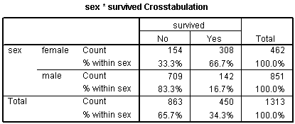
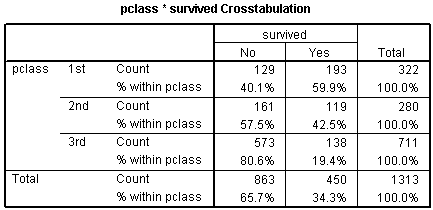
Both the odds ratio and the relative risk compare the likelihood of an event between two groups. Consider the following data on survival of passengers on the Titanic. There were 462 female passengers: 308 survived and 154 died. There were 851 male passengers: 142 survived and 709 died (see table below).
Alive Dead Total Female 308 154 462 Male 142 709 851 Total 450 863 1,313
Clearly, a male passenger on the Titanic was more likely to die than a female passenger. But how much more likely? You can compute the odds ratio or the relative risk to answer this question.
The odds ratio compares the relative odds of death in each group. For females, the odds were exactly 2 to 1 against dying (154/308=0.5). For males, the odds were almost 5 to 1 in favor of death (709/142=4.993). The odds ratio is 9.986 (4.993/0.5). There is a ten fold greater odds of death for males than for females.
The relative risk (sometimes called the risk ratio) compares the probability of death in each group rather than the odds. For females, the probability of death is 33% (154/462=0.3333). For males, the probability is 83% (709/851=0.8331). The relative risk of death is 2.5 (0.8331/0.3333). There is a 2.5 greater probability of death for males than for females.
There is quite a difference. Both measurements show that men were more likely to die. But the odds ratio implies that men are much worse off than the relative risk. Which number is a fairer comparison?
There are three issues here: The relative risk measures events in a way that is interpretable and consistent with the way people really think. The relative risk, though, cannot always be computed in a research design. Also, the relative risk can sometimes lead to ambiguous and confusing situations. But first, we need to remember that fractions are funny.
Fractions are funny.
Suppose you invested money in a stock. On the first day, the value of the stock decreased by 20%. On the second day it increased by 20%. You would think that you have broken even, but that's not true.
Take the value of the stock and multiply by 0.8 to get the price after the first day. Then multiply by 1.2 to get the price after the second day. The successive multiplications do not cancel out because 0.8 * 1.2 = 0.96. A 20% decrease followed by a 20% increase leaves you slightly worse off.
It turns out that to counteract a 20% decrease, you need a 25% increase. That is because 0.8 and 1.25 are reciprocal. This is easier to see if you express them as simple fractions: 4/5 and 5/4 are reciprocal fractions. Listed below is a table of common reciprocal fractions.
0.8 (4/5) 1.25 (5/4) 0.75 (3/4) 1.33 (4/3) 0.67 (2/3) 1.50 (3/2) 0.50 (1/2) 2.00 (2/1) Sometimes when we are comparing two groups, we'll put the first group in the numerator and the other in the denominator. Sometimes we will reverse ourselves and put the second group in the numerator. The numbers may look quite different (e.g., 0.67 and 1.5) but as long as you remember what the reciprocal fraction is, you shouldn't get too confused.
For example, we computed 2.5 as the relative risk in the example above. In this calculation we divided the male probability by the female probability. If we had divided the female probability by the male probability, we would have gotten a relative risk of 0.4. This is fine because 0.4 (2/5) and 2.5 (5/2) are reciprocal fractions.
Interpretability
The most commonly cited advantage of the relative risk over the odds ratio is that the former is the more natural interpretation.
The relative risk comes closer to what most people think of when they compare the relative likelihood of events. Suppose there are two groups, one with a 25% chance of mortality and the other with a 50% chance of mortality. Most people would say that the latter group has it twice as bad. But the odds ratio is 3, which seems too big. The latter odds are even (1 to 1) and the former odds are 3 to 1 against.
Even more extreme examples are possible. A change from 25% to 75% mortality represents a relative risk of 3, but an odds ratio of 9.
A change from 10% to 90% mortality represents a relative risk of 9 but an odds ratio of 81.
There are some additional issues about interpretability that are beyond the scope of this paper. In particular, both the odds ratio and the relative risk are computed by division and are relative measures. In contrast, absolute measures, computed as a difference rather than a ratio, produce estimates with quite different interpretations (Fahey et al 1995, Naylor et al 1992).
Designs that rule out the use of the relative risk
Some research designs, particularly the case-control design, prevent you from computing a relative risk. A case-control design involves the selection of research subjects on the basis of the outcome measurement rather than on the basis of the exposure.
Consider a case-control study of prostate cancer risk and male pattern balding. The goal of this research was to examine whether men with certain hair patterns were at greater risk of prostate cancer. In that study, roughly equal numbers of prostate cancer patients and controls were selected. Among the cancer patients, 72 out of 129 had either vertex or frontal baldness compared to 82 out of 139 among the controls (see table below).
Cancer cases Controls Total Balding 72 82 154 Hairy 55 57 112 Total 129 139 268
In this type of study, you can estimate the probability of balding for cancer patients, but you can't calculate the probability of cancer for bald patients. The prevalence of prostate cancer was artificially inflated to almost 50% by the nature of the case-control design.
So you would need additional information or a different type of research design to estimate the relative risk of prostate cancer for patients with different types of male pattern balding. Contrast this with data from a cohort study of male physicians (Lotufo et al 2000). In this study of the association between male pattern baldness and coronary heart disease, the researchers could estimate relative risks, since 1,446 physicians had coronary heart disease events during the 11-year follow-up period.
For example, among the 8,159 doctors with hair, 548 (6.7%) developed coronary heart disease during the 11 years of the study. Among the 1,351 doctors with severe vertex balding, 127 (9.4%) developed coronary heart disease (see table below). The relative risk is 1.4 = 9.4% / 6.7%.
Heart disease Healthy Total Balding 127 (9.4%) 1,224 (90.6%) 1,351 Hairy 548 (6.7%) 7,611 (93.3%) 8,159 Total 675 8,835 9,510
You can always calculate and interpret the odds ratio in a case control study. It has a reasonable interpretation as long as the outcome event is rare (Breslow and Day 1980, page 70). The interpretation of the odds ratio in a case-control design is, however, also dependent on how the controls were recruited (Pearce 1993).
Another situation which calls for the use of odds ratio is covariate adjustment. It is easy to adjust an odds ratio for confounding variables; the adjustments for a relative risk are much trickier.
In a study on the likelihood of pregnancy among people with epilepsy (Schupf and Ottman 1994), 232 out of 586 males with idiopathic/cryptogenic epilepsy had fathered one or more children. In the control group, the respective counts were 79 out of 109 (see table below).
Children No children Total Epilepsy 232 (40%) 354 (60%) 586 Control 79 (72%) 30 (28%) 109 Total 311 384 695
The simple relative risk is 0.55 and the simple odds ratio is 0.25. Clearly the probability of fathering a child is strongly dependent on a variety of demographic variables, especially age (the issue of marital status was dealt with by a separate analysis). The control group was 8.4 years older on average (43.5 years versus 35.1), showing the need to adjust for this variable. With a multivariate logistic regression model that included age, education, ethnicity and sibship size, the adjusted odds ratio for epilepsy status was 0.36. Although this ratio was closer to 1.0 than the crude odds ratio, it was still highly significant. A comparable adjusted relative risk would be more difficult to compute (although it can be done as in Lotufo et al 2000).
Ambiguous and confusing situations
The relative risk can sometimes produce ambiguous and confusing situations. Part of this is due to the fact that relative measurements are often counter-intuitive. Consider an interesting case of relative comparison that comes from a puzzle on the Car Talk radio show. You have a hundred pound sack of potatoes. Let's assume that these potatoes are 99% water. That means 99 parts water and 1 part potato. These are soggier potatoes than I am used to seeing, but it makes the problem more interesting.
If you dried out the potatoes completely, they would only weigh one pound. But let's suppose you only wanted to dry out the potatoes partially, until they were 98% water. How much would they weigh then?
The counter-intuitive answer is 50 pounds. 98% water means 49 parts water and 1 part potato. An alternative way of thinking about the problem is that in order to double the concentration of potato (from 1% to 2%), you have to remove about half of the water.
Relative risks have the same sort of counter-intuitive behavior. A small relative change in the probability of a common event's occurrence can be associated with a large relative change in the opposite probability (the probability of the event not occurring).
Consider a recent study on physician recommendations for patients with chest pain (Schulman et al 1999). This study found that when doctors viewed videotape of hypothetical patients, race and sex influenced their recommendations. One of the findings was that doctors were more likely to recommend cardiac catheterization for men than for women. 326 out of 360 (90.6%) doctors viewing the videotape of male hypothetical patients recommended cardiac catheterization, while only 305 out of 360 (84.7%) of the doctors who viewed tapes of female hypothetical patients made this recommendation.
No cath Cath Total Male patient 34 (9.4%) 326 (90.6%) 360 Female patient 55 (15.3%) 305 (84.7%) 360 Total 89 631 720
The odds ratio is either 0.57 or 1.74, depending on which group you place in the numerator. The authors reported the odds ratio in the original paper and concluded that physicians make different recommendations for male patients than for female patients.
A critique of this study (Schwarz et al 1999) noted among other things that the odds ratio overstated the effect, and that the relative risk was only 0.93 (reciprocal 1.07). In this study, however, it is not entirely clear that 0.93 is the appropriate risk ratio. Since 0.93 is so much closer to 1 and 0.57, the critics claimed that the odds ratio overstated the tendency for physicians to make different recommendations for male and female patients.
Although the relative change from 90.6% to 84.7% is modest, consider the opposite perspective. The rates for recommending a less aggressive intervention than catheterization was 15.3% for doctors viewing the female patients and 9.4% for doctors viewing the male patients, a relative risk of 1.63 (reciprocal 0.61).
This is the same thing that we just saw in the Car Talk puzzler: a small relative change in the water content implies a large relative change in the potato content. In the physician recommendation study, a small relative change in the probability of a recommendation in favor of catheterization corresponds to a large relative change in the probability of recommending against catheterization.
Thus, for every problem, there are two possible ways to compute relative risk. Sometimes, it is obvious which relative risk is appropriate. For the Titanic passengers, the appropriate risk is for death rather than survival. But what about a breast feeding study. Are we trying to measure how much an intervention increases the probability of breast feeding success or are we trying to see how much the intervention decreases the probability of breast feeding failure? For example, Deeks 1998 expresses concern about an odds ratio calculation in a study aimed at increasing the duration of breast feeding. At three months, 32/51 (63%) of the mothers in the treatment group had stopped breast feeding compared to 52/57 (91%) in the control group.
Continued bf Stopped bf Total Treatment 19 (37.3%) 32 (62.7%) 51 Control 5 (8.8%) 52 (91.2%) 57 Total 24 84 108
While the relative risk of 0.69 (reciprocal 1.45) for this data is much less extreme than the odds ratio of 0.16 (reciprocal 6.2), one has to wonder why Deeks chose to compare probabilities of breast feeding failures rather than successes. The rate of successful breast feeding at three months was 4.2 times higher in the treatment group than the control group. This is still not as extreme as the odds ratio; the odds ratio for successful breast feeding is 6.25, which is simply the inverse of the odds ratio for breast feeding failure.
One advantage of the odds ratio is that it is not dependent on whether we focus on the event's occurrence or its failure to occur. If the odds ratio for an event deviates substantially from 1.0, the odds ratio for the event's failure to occur will also deviate substantially from 1.0, though in the opposite direction.
Summary
Both the odds ratio and the relative risk compare the relative likelihood of an event occurring between two distinct groups. The relative risk is easier to interpret and consistent with the general intuition. Some designs, however, prevent the calculation of the relative risk. Also there is some ambiguity as to which relative risk you are comparing. When you are reading research that summarizes the data using odds ratios, or relative risks, you need to be aware of the limitations of both of these measures.
Bibliography
When can odds ratios mislead? Odds ratios should be used only in case-control studies and logistic regression analyses [letter]. Deeks J. British Medical Journal 1998:317(7166);1155-6; discussion 1156-7.
Evidence-based purchasing: understanding results of clinical trials and systematic reviews. Fahey T, Griffiths S and Peters TJ. British Medical Journal 1995:311(7012);1056-9; discussion 1059-60.
Interpretation and Choice of Effect Measures in Epidemiologic Analyses. Greenland S. American Journal of Epidemiology 1987:125(5);761-767.
Male Pattern Baldness and Coronary Heart Disease: The Physician's Health Study. Lotufo PA. Archives of Internal Medicine 2000:160(165-171.
Measured Enthusiasm: Does the Method of Reporting Trial Results Alter Perceptions of Therapeutic Effectiveness? Naylor C, Chen E and Strauss B. American College of Physicians 1992:117(11);916-21.
What Does the Odds Ratio Estimate in a Case-Control Study? Pearce N. Int J Epidemiol 1993:22(6);1189-92.
Likelihood of Pregnancy in Individuals with Idiopathic/Cryptogenic Epilepsy: Social and Biologic Influences. Schupf N. Epilepsia 1994:35(4);750-756.
A Haircut in Horse Town: And Other Great Car Talk Puzzlers. (1999) Tom Magliozzi, Ray Magliozzi, Douglas Berman. New York NY: Berkley Publishing Group.
This webpage was written by Steve Simon on (2001-01-09), edited by Steve Simon, and was last modified on 2008-07-08.
The concepts behind the logistic regression model (July 23, 2002)
The logistic regression model is a model that uses a binary (two possible values) outcome variable. Examples of a binary variable are mortality (live/dead), and morbidity (healthy/diseased). Sometimes you might take a continuous outcome and convert it into a binary outcome. For example, you might be interested in the length of stay in the hospital for mothers during an unremarkable delivery. A binary outcome might compare mothers who were discharged within 48 hours versus mothers discharged more than 48 hours.
The covariates in a logistic regression model represent variables that might be associated with the outcome variable. Covariates can be either continuous or categorical variables.
For binary outcomes, you might find it helpful to code the variable using indicator variables. An indicator variable equals either zero or one. Use the value of one to represent the presence of a condition and zero to represent absence of that condition. As an example, let 1=diseased, 0=healthy.
Indicator variables have many nice mathematical properties. One simple property is that the average of an indicator variable equals the observed probability in your data of the specific condition for that variable.
A logistic regression model examines the relationship between one or more independent variable and the log odds of your binary outcome variable. Log odds seem like a complex way to describe your data, but when you are dealing with probabilities, this approach leads to the simplest description of your data that is consistent with the rules of probability.
Let's consider an artificial data example where we collect data on the gestational age of infants (GA), which is a continuous variable, and the probability that these infants will be breast feeding at discharge from the hospital (BF), which is a binary variable. We expect an increasing trend in the probability of BF as GA increases. Premature infants are usually sicker and they have to stay in the hospital longer. Both of these present obstacles to BF.
A linear model for probability
A linear model would presume that the probability of BF increases as a linear function of GA. You can represent a linear function algebraically as
prob BF = a + b*GA
This means that each unit increase in GA would add b percentage points to the probability of BF. The table shown below gives an example of a linear function.
This table represents the linear function
prob BF = 4 + 2*GA
which means that you can get the probability of BF by doubling GA and adding 4. So an infant with a gestational age of 30 would have a probability of 4+2*30 = 64.
A simple interpretation of this model is that each additional week of GA adds an extra 2% to the probability of BF. We could call this an additive probability model.
I'm not an expert on BF; what little experience I've had with the topic occurred over 40 years ago. But I do know that an additive probability model tends to have problems when you get probabilities close to 0% or 100%. Let's change the linear model slightly to the following:
prob BF = 4 + 3*GA
This model would produce the following table of probabilities.
You may find it difficult to explain what a probability of 106% means. This is a reason to avoid using a additive model for estimating probabilities. In particular, try to avoid using an additive model unless you have good reason to expect that all of your estimated probabilities will be between 20% and 80%.
A multiplicative model for probability
It's worthwhile to consider a different model here, a multiplicative model for probability, even though it suffers from the same problems as the additive model.
In a multiplicative model, you change the probabilities by multiplying rather than adding. Here's a simple example.
In this example, each extra week of GA produces a tripling in the probability of BF. Contrast this to the linear models shown above, where each extra week of GA adds 2% or 3% to the probability of BF.
A multiplicative model can't produce any probabilities less than 0%, but it's pretty easy to get a probability bigger than 100%. A multiplicative model for probability is actually quite attractive, as long as you have good reason to expect that all of the probabilities are small, say less than 20%.
The relationship between odds and probability
Another approach is to try to model the odds rather than the probability of BF. You see odds mentioned quite frequently in gambling contexts. If the odds are three to one in favor of your favorite football team, that means you would expect a win to occur about three times as often as a loss. If the odds are four to one against your team, you would expect a loss to occur about four times as often as a win.
You need to be careful with odds. Sometimes the odds represent the odds in favor of winning and sometimes they represent the odds against winning. Usually it is pretty clear from the context. When you are told that your odds of winning the lottery are a million to one, you know that this means that you would expect to having a losing ticket about a million times more often than you would expect to hit the jackpot.
It's easy to convert odds into probabilities and vice versa. With odds of three to one in favor, you would expect to see roughly three wins and only one loss out of every four attempts. In other words, your probability for winning is 0.75.
If you expect the probability of winning to be 20%, you would expect to see roughly one win and four losses out of every five attempts. In other words, your odds are 4 to 1 against.
The formulas for conversion are
odds = prob / (1-prob)
and
prob = odds / (1+odds).
In medicine and epidemiology, when an event is less likely to happen and more likely not to happen, we represent the odds as a value less than one. So odds of four to one against an event would be represented by the fraction 1/4 or 0.25. When an event is more likely to happen than not, we represent the odds as a value greater than one. So odds of three to one in favor of an event would be represented simply as an odds of 3. With this convention, odds are bounded below by zero, but have no upper bound.
A log odds model for probability
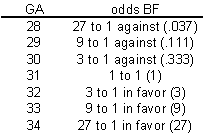
Let's consider a multiplicative model for the odds (not the probability) of BF.
This model implies that each additional week of GA triples the odds of BF. A multiplicative model for odds is nice because it can't produce any meaningless estimates.
It's interesting to look at how the logarithm of the odds behave.
Notice that an extra week of GA adds 1.1 units to the log odds. So you can describe this model as linear (additive) in the log odds. When you run a logistic regression model in SPSS or other statistical software, it uses a model just like this, a model that is linear on the log odds scale. This may not seem too important now, but when you look at the output, you need to remember that SPSS presents all of the results in terms of log odds. If you want to see results in terms of probabilities instead of logs, you have to transform your results.
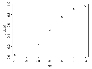
Let's look at how the probabilities behave in this model.
Notice that even when the odds get as large as 27 to 1, the probability still stays below 100%. Also notice that the probabilities change in neither an additive nor a multiplicative fashion.
A graph shows what is happening.
The probabilities follow an S-shaped curve that is characteristic of all logistic regression models. The curve levels off at zero on one side and at one on the other side. This curve ensures that the estimated probabilities are always between 0% and 100%.
An example of a log odds model with real data
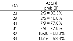
There are other approaches that also work well for this type of data, such as a probit model, that I won't discuss here. But I did want to show you what the data relating GA and BF really looks like.
I've simplified this data set by removing some of the extreme gestational ages. The estimated logistic regression model is
log odds = -16.72 + 0.577*GA
The table below shows the predicted log odds, and the calculations needed to transform this estimate back into predicted probabilities.
Let's examine these calculations for GA = 30. The predicted log odds would be
log odds = -16.72 + 0.577*30 = 0.59
Convert from log odds to odds by exponentiating.
odds = exp(0.59) = 1.80
And finally, convert from odds back into probability.
prob = 1.80 / (1+1.80) = 0.643
The predicted probability of 64.3% is reasonably close to the true probability (77.8%).
You might also want to take note of the predicted odds. Notice that the ratio of any odds to the odds in the next row is 1.78. For example,
3.20/1.80 = 1.78
5.70/3.20 = 1.78
It's not a coincidence that you get the same value when you exponentiate the slope term in the log odds equation.
exp(0.59) = 1.78
This is a general property of the logistic model. The slope term in a logistic regression model represents the log of the odds ratio representing the increase (decrease) in risk as the independent variable increases by one unit.
Categorical variables in a logistic regression model
You treat categorical variables in much the same way as you would in a linear regression model. Let's start with some data that listed survival outcomes on the Titanic. That ship was struck by an iceberg and 863 passengers died out of a total of 1,313. This happened during an era where there was a strong belief in "women and children" first.
You can see this in the crosstabulation shown above. Among females, the odds of dying were 2-1 against, because the number of survivors (308) was twice as big as the number who died (154). Among males, the odds of dying were almost 5 to 1 in favor (actually 4.993 to 1), since the number who survived (142) was about one-fifth the number who died (709).
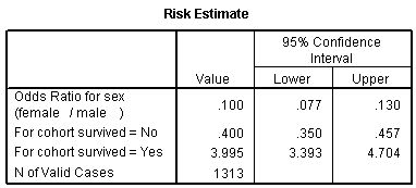
The odds ratio is 0.1, and we are very confident that this odds ratio is less than one, because the confidence interval goes up to only 0.13. Let's analyze this data by creating an indicator variable for sex.
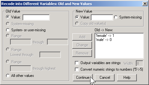
In SPSS, you would do this by selecting TRANSFORM | RECODE from the menu
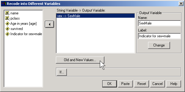
Then click on the OLD AND NEW VALUES button.
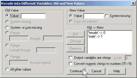
Here, I use the codes of 0 for female and 1 for male. To run a logistic regression in SPSS, select ANALYZE | REGRESSION | BINARY LOGISTIC from the menu.
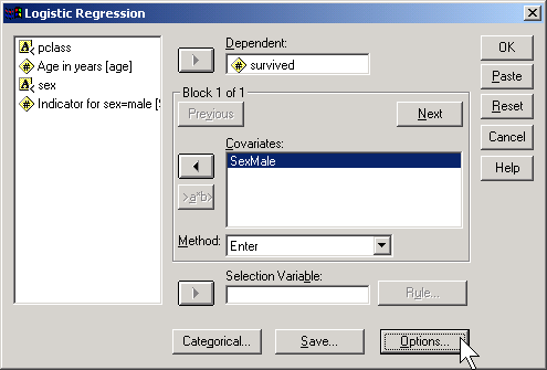
Click on the OPTIONS button.
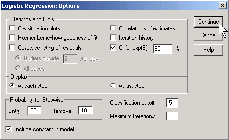
Select the CI for exp(B) option, then click on the CONTINUE button and then on the OK button. Here is what the output looks like:
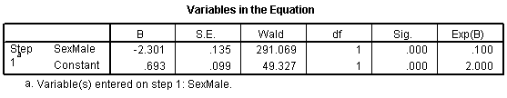
Let's start with the CONSTANT row of the data. This has an interpretation similar to the intercept in the linear regression model. the B column represents the estimated log odds when SexMale=0. Above, you saw that the odds for dying were 2 to 1 against for females, and the natural logarithm of 2 is 0.693. The last column, EXP(B) represents the odds, or 2.000. You need to be careful with this interpretation, because sometimes SPSS will report the odds in favor of an event and sometimes it will report the odds against an event. You have to look at the crosstabulation to be sure which it is.
The SexMale row has an interpretation similar to the slope term in a linear regression model. The B column represents the estimated change in the log odds when SexMale increases by one unit. This is effectively the log odds ratio. We computed the odds ratio above, and -2.301 is the natural logarithm of 0.1. The last column, EXP(B) provides you with the odds ratio (0.100).
Coding is very important here. Suppose you had chosen the coding for SexFemale where1=female and 0=male.
Then the output would look quite different.
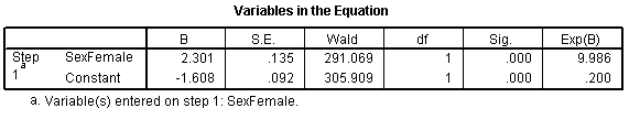
The log odds is now -1.608 which represents the log odds for males. The log odds ratio is now 2.301 and the odds ratio is 9.986 (which you might want to round to 10).
SPSS will create an indicator variable for you if you click on the CATEGORICAL button in the logistic regression dialog box.
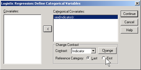
If you select LAST as the reference category, SPSS will use the code 0=male, 1=female (last means last alphabetically). If you select FIRST as the reference category, SPSS will use the code 0=female, 1=male.
How would SPSS handle a variable like Passenger Class, which has three levels
- 1st,
- 2nd,
- 3rd?
Here's a crosstabulation of survival versus passenger class.
Notice that the odds of dying are 0.67 to 1 in 1st class, 1.35 to 1 in 2nd class, and 4.15 to 1 in 3rd class. These are odds in favor of dying. The odds against dying are 1.50 to 1, 0.74 to 1, and 0.24 to 1, respectively.
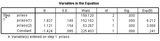
The odds ratio for the pclass(1) row is 6.212, which is equal to 1.50 / 0.24. You should interpret this as the odds against dying are 6 times better in first class compared to third class. The odds ratio for the pclass(2) row is 3.069, which equals 0.74 / 0.24. This tells you that the odds against dying are about 3 times better in second class compared to third class. The Constant row tells you that the odds are 0.241 to 1 in third class.
If you prefer to do the analysis with each of the other classes being compared back to first class, then select FIRST for reference category.
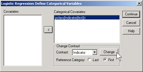
This produces the following output:
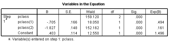
Here the pclass(1) row provides an odds ratio of 0.494 which equals 0.74 / 1.50. The odds against dying are about half in second class versus first class. The pclass(2) provides an odds ratio of 0.161 (approximately 1/6) which equals 0.24 / 1.50. The odds against dying are 1/6 in third class compared to first class. The Constant row provides an odds of 1.496 to 1 against dying for first class.
Notice that the numbers in parentheses (pclass(1) and pclass(2)) do not necessarily correspond to first and second classes. It depends on how SPSS chooses the indicator variables. How did I know how to interpret the indicator variables and the odds ratios? I wouldn't have known how to do this if I hadn't computed a crosstabulation earlier. It is very important to do a few simple crosstabulations before you run a logistic regression model, because it helps you orient yourself to the data.
Looking at a variable both continuously and categorically.
Suppose you wanted to further explore the concept of "women and children first" by looking at how age affects the odds against survival. Here is a simple model that includes age as a continuous variable:
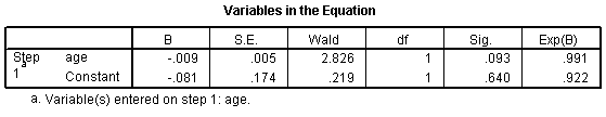
The odds ratio for age is 0.991. This tells you that the odds against dying drop by about 1% for each year of life. In other words, the older you are the more likely you are to die. Let's re-interpret this in terms of decades. A full decade change in age would lead to a -0.009 * 10 unit change in the log odds ratio. This leads to an odds ratio of 0.91 per decade, which says the odds against dying decline by about 9% for each extra decade of life.
I have a problem with this model, because it assumes that the effect of one year of age is the same for children, teenagers, adults, and very old people. I suspect that perhaps the effect of age is very strong for young people but it levels off in adults. The chances of dying for a 30 year old would probably not be too much different than for a 40 year old. Let's split the data into different age groups and see how each of them compares.
To do this in SPSS, select TRANSFORM | RANK CASES from the menu.

Click on the RANK TYPES button.
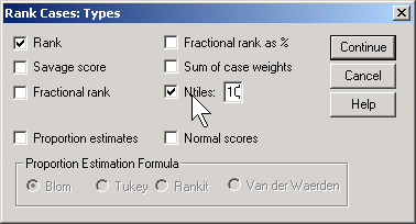
Select Ntiles and choose 10 for the number of groups. This is a somewhat arbitrary choice. You want enough groups to allow for subtle changes across the age range, but if there are too many groups, you lose too much precision.
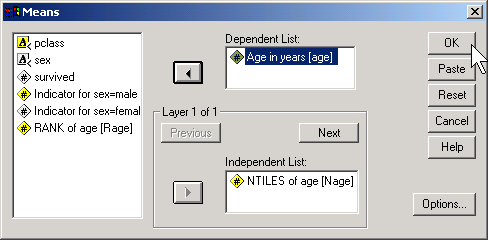
Here's what you get

Notice that the first group has an average age of 6.6. We'll call those the young children. The next group has an average age of 17.9 which looks more like older teenagers. The remaining groups represent adults of various ages. We have about 70-80 people in each age group. Here is a crosstabulation of age groups by survival.
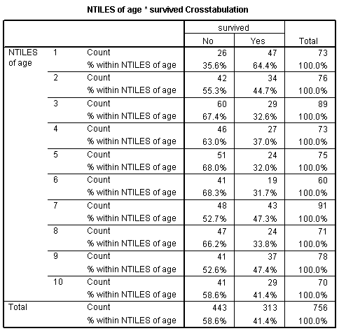
Notice that the chances for survival are best for the young children. Survival also seems to be high for older teenagers and some of the older adult categories. The worst survival rates are in age groups 3, 4, 5, 6, and 8. Perhaps there is some tendency in this data for "women, children, and old people" first. Here's what a logistic regression model looks like for age groups.

All age groups have a decreased chance of surviving relative to the young children group. You might want to investigate this further looking at combining some or all of the adult groups and splitting the young children group into further subcategories.
This webpage was written by Steve Simon and was last modified on 07/08/2008.
What does "overfitting" mean? (July 24, 2003)
Dear Professor Mean, I am conducting binary logistic regression analyses with a sample size of 80 of which 20 have the outcome of interest (e.g. are "very successful" versus somewhat/not very successful). I have thirty possible independent variables which I examined in a univariate logistic regression with the dependent variable. Of these thirty, five look like they might have a relationship with the independent variable. Now I want to include these six variables in a stepwise logistic regression model, but I am worried about overfitting the data. I have heard that there should be about 10 cases with the outcome of interest per independent variable to avoid overfitting. What exactly does overfitting mean?
I apologize if some of the comments here appear harsh. You are going to have to seriously lower your expectations. That may be disheartening, but better to face the bad news now rather than later.
What is overfitting?
Overfitting means that some of the relationships that appear statistically significant are actually just noise. It occurs when the complexity of the statistical model is too great for the amount of data that you have. You will find that a model with overfitting does not replicate well and does a lousy job of predicting future responses. In simple words, the model stinks.
Rule of ten observations per variable.
The rule of 10 observations per variable (I've also heard 15) is referring to the number of variables screened, not the number in the final model. Since you looked at 30 variables, you really needed 300 to 450 events of interest to be sure that your model is not overfitting the data.
What to do, what to do?
If you are trying to publish these results, you have to hope that the reviewers are all asleep at the switch. Instead of a ratio of 10 or 15 to one, your ratio is less than one to one. You have more variables than events. And since all 30 variables are part of the initial screen, so you can't say that you only looked at 5 variables.
Of course, you were unfortunate enough to have the IRB asleep at the switch, because they should never have approved such an ambitious data analysis on such a skimpy data set. So maybe the reviewers will be the same way.
I wouldn't count on it, though. If you want to improve your chances of publishing the results, there are several things you can do.
1. I realize that the answer is almost always "NO" but I still have to ask--is there any possibility that you could collect more data? In theory, collecting more data after the study has ended is a protocol deviation (be sure to tell your IRB). And there is some possibility of temporal trends that might interfere with your logistic model. But both of these "sins" are less serious than overfitting your data.
2. You could slap the "exploratory" label on your research. Put in a lot of qualifiers like "Although these results are intriguing, the small sample size means that these results may not replicate well with a larger data set." This is a cop-out in my opinion. I've fallen back on this when I've seen ratios of four to one or three to one, but you don't even come close to those ratios.
3. Ask a colleague who has not looked at the data to help. Show him/her the list of 30 independent variables and ask which two should be the highest priority, based on biological mechanisms, knowledge of previous research, intuition, etc., BUT NOT LOOKING AT THE EXISTING DATA. Then do a serious logistic regression model with those two variables, and treat the other twelve variables in a purely exploratory mode.
4. Admit to yourself that you are trying to squeeze blood from a turnip. A sample of 80 with only 20 events of interest is just not big enough to allow for a decent multivariable logistic regression model. You can't look for the effect of A, adjusted for B, C, and D, so don't even try. Report each individual univariate logistic regression model and leave it at that.
5. Give up all thoughts of logistic regression and p-values altogether. This may seem like a radical approach, but who made a rule that says that every research publication has to have p-values? Submit a publication with a graphical summary of your data. Boxplots and/or bar charts would work very nicely here. Explain that your data set is too small to entertain any serious logistic regression models. If you're unlucky, then the reviewers may ask you to put in some p-values anyway. Then you could switch to the previous option.
6. There are some newer approaches to statistical modeling that are less prone to overfitting. Perhaps the one you are most likely to see if CART (Classification and Regression Trees). These models can't make a silk purse out of a sow's ear, but they do have some cross validation checks that make them slightly better than stepwise approaches.
Summary
If you asked a group of statisticians how many of them have published results when they knew that the sample size was way too small, almost every hand would go up, I suspect. I've done it more times than I want to admit. Just be sure to scale back your expectations, limit the complexity of any models, and be honest about the limitations of your sample size.
This webpage was written by Steve Simon on 2003-07-23, edited by Steve Simon, and was last modified on 2008-07-08.
Guidelines for logistic regression models (September 27, 1999)
There are three steps in a typical logistic regression model.
Step 1. Fit a crude model.
There are two types of models, crude models and adjusted models. A crude model looks at how a single factor affects your outcome measure and ignores potential covariates. An adjusted model incorporates these potential covariates. Start with a crude model. It's simpler and it helps you to get a quick overview of how things are panning out. Then continue by making adjustments for important confounders.
If the factor that you use to predict your binary outcome is itself binary, you can visualize how the logistic regression model works by arranging your data in a two by two table.

In this example, the treatment group (also labeled "ng tube" in other parts of this website) represents a group of children who received feeding by ng tube when the mother was not in the hospital while the control group (also labeled "bottle" in other parts of this website) received bottles when the mother was not in the hospital.
The Feeding type * Exclusive bf at discharge Crosstabulation shows us the frequency for the four possible combinations of feeding type and breast feeding status at discharge. It helps to also look at the row percentages and the risk option.

The table above shows row percentages for the exclusive breast feeding status at discharge. Notice that a much greater fraction of the Treatment group were exclusive breast feeding at discharge (86.8% versus 41.3% for the control group).

The Risk Estimate table appears when we select the RISK option. This table provides information about the odds ratio and two different risk ratios. The odds ratio is 9.379. You should always be careful about this estimate, because it is dependent on how we arrange the table. If we reversed the rows, for example, and placed the NG Tube group on top, the odds ratio would be inverted. We would have an odds ratio of of 0.107 (=1/9.379). If an odds ratio seems inconsistent with your previous results, be sure to compute the inverse and see if that is consistent.
Notice that SPSS provides two additional estimates. These two additional estimates are risk ratios and are computed by dividing one row percentage by the other. The value of 4.461 is the ratio of 58.7% divided by 13.2%. This is the increase in the probability of not exclusively breast feeding at discharge when we compare the NG Tube group to the Bottle Fed group.
The other estimate, 0.476 (= 41.3/86.8), represents the change in the probability of exclusive breast feeding when we compare the NG Tube group to the Bottle Fed group.
The logistic regression output from SPSS is quite extensive. We will break it apart into pieces and discuss each piece individually.

The Case Processing Summary table shows you information on missing cases and unselected cases. Make sure that you are not losing data unexpectedly.

The Dependent Variable Encoding table shows you which of the categories is labeled as 0 and which is labeled as 1. If the estimates that you get later in the output go in the opposite direction from what you would expect, check here to see if the encoding is reversed from what you expected.
We will skip any discussion of all of the tables in Step 0. These represent the status of a null model with no independent variables other than an intercept. These values are more likely to be interesting if you are fitting a sequential series of logistic regression models.

The Omnibus Tests of Model Coefficients table is mostly of interest for more complex logistic regression models. It provides a test of the joint predictive ability of all the covariates in the model.

The Model Summary table in Step 1 shows three measures of how well the logistic regression model fits the data. These measures are useful when you are comparing several different logistic regression models.

The Classification Table in Step1 is often useful for logistic regression models which involve diagnostic testing, but you usually have to set the Classification Cut-off field to a value other than the default of 0.5. You might want to try instead to use the prevalence of disease in your sample as your cut-off. Under certain circumstances, the percentage correct could relate to sensitivity and specificity (or the reverse), though the use of these terms is a bit unusual for a breast feeding study since this represents a condition not related to disease.
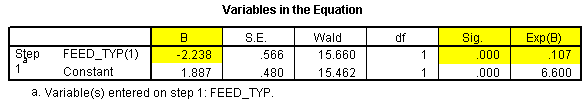
In the Variables in the Equation table for Step 1, the B column represents the estimated log odds ratio. The Sig. column represents the p-value for testing whether feeding type is significantly associated with exclusive breast feeding at discharge. The Exp(B) column represents the odds ratio. Notice that this odds ratio (0.107) is quite a bit different than the one computed using the crosstabulation (9.379). But it is just the inverse; check it out on your own calculator.
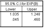
We can also get a confidence interval for the odds ratio by clicking on the Options button and selecting the the CI for exp(B) option box.

If we were interested in the earlier odds ratio of 9.379 instead of 0.107, then we would compute the reciprocal of the confidence limits. Thus 3.1 (=1/0.323) and 28.6 (=1/0.035) represent 95% confidence limits.
Let's look at another logistic regression model, where we try to predict exclusive breast feeding at discharge using the mother's age as a continuous covariate.

The log odds ratio is 0.157 and the p-value is 0.001. The odds ratio is 1.170. This implies that the estimated odds of successful breast feeding at discharge improve by about 17% for each additional year of the mother's age.

The confidence limit is 1.071 to 1.278, which tells you that even after allowing for sampling error, the estimated odds will increase by at least 7% for each additional year of age.
If you wanted to see how much the odds would change for each additional five years of age, take the odds ratio and raise it to the fifth power. This gets you a value of 2.19, which implies that a change of five years in age will more than double the odds of exclusive breast feeding.
Step 2. Fit an adjusted model
The crude model shown in step 1, tells you that the odds of breast feeding is nine times higher in the ng tube group than in the bottle group. A previous descriptive analysis, however, told you that older mothers were more likely to be in the ng tube group and younger mothers were more likely to be in the bottle fed group. This was in spite of randomization. So you may wish to see how much of the impact of feeding type on breast feeding can be accounted for by the discrepancy in mothers' ages. This is an adjusted logistic model.
When you run this model, put FEED_TYP as a covariate in the first block and put MOM_AGE as a covariate in the second block. The full output has much in common with the output for the crude model. Important excerpts appear below.

The Omnibus Tests of Model Coefficients table and the Model Summary table for Block 1 are identical to those in the crude model with MOM_AGE as the covariate. We wish to contrast these with the same tables for Block 2.

The Chi-square values in the Omnibus Tests of Model Coefficients table in Block 2 show some changes.
The test in the Model row shows the predictive power of all of the variables in Block 1 and Block 2. The large Chi-square value (28.242) and the small p-value (0.000) show you that either feeding type or mother's age or both are significantly associated with exclusive breast feeding at discharge.
The test in the Block row represents a test of the predictive power of all the variables in Block 2, after adjusting for all the variables in Block 1. The large Chi-square value (12.398) and the small p-value (0.000) indicates that feeding type is significantly associated with exclusive breast feeding at discharge, even after adjusting for mother's age. The Chi-square value is computed as the difference between the -2 Log likelihood at Block 1 (95.797) and Block 2 (83.399).
Notice that the two R-squared measures are larger. This also tells you that feeding type helps in predicting breastfeeding outcome, above and beyond mother's age.

The odds ratio for mother's age is 1.1367. That tells you that each for additional year of the mother's age, the odds of breast feeding increase by 1.14 (or 14%), assuming that the feeding type is held constant.
The odds ratio for feeding type is 0.1443 or, if we invert it, 6.9. This tells us that the odds for breast feeding are about 7 times great in the ng tube group than in the bottle fed group, assuming that mother's age is held constant. Notice that the effect of feeding type adjusting for mother's age is not quite as large as the crude odds ratio, but it is still large and it still is statistically significant (the p-value is .001 and the confidence interval excludes the value of 1.0).
Step 3. Examine the predicted probabilities.
The logistic regression model produces estimated or predicted probabilities and we should compare these to probabilities observed in the data. A large discrepancy indicates that you should look more closely at your data and possibly consider some alternative models.
If you coded your outcome variable as 0 and 1, then you can compute the average to get probabilities observed in the data. But if you have a lot of values for your covariate, you have to group it first.

The Report table shows average predicted probabilities (Predicted probability column) and observed probabilities (Exclusive bf at discharge column) for mother's age. We had to create a new variable where we created five groups of roughly equal size. The first group represented the 15 mothers with the youngest ages and the fifth group represented the 17 mothers with the oldest ages. The last column (Mother's age column) shows the average age in each of the five groups.

The Hosmer and Lemeshow Test table provides a formal test for whether the predicted probabilities for a covariate match the observed probabilities. A large p-value indicates a good match. A small p-value indicates a poor match, which tells you that you should look for some alternative ways to describe the relationship between this covariate and the outcome variable. In our example, the p-value is large (0.545), indicating a good match.

The Contingency Table for Hosmer and Lemeshow Test table shows more details. This test divides your data up into approximately ten groups. These groups are defined by increasing order of estimated risk. The first group corresponds to those subjects who have the lowest predicted risk. In this model it represents the seven subjects where the mother's age is 16, 17, or 18 years. Notice that in this group of 16-18 year old mothers, six were not successful BF and one was. This corresponds to the observed counts in the first three rows of the Mother's age * Exclusive bf at discharge Crosstabulation table (shown below, with the bottom half editted out). The second group of eight mothers represents 19 and 20 year olds, where 4 were exclusive breast feeding at discharge. The third group represents nine mothers aged 21 and 22 years old, and so forth.

The next group corresponds to those with the next lowest risk, those mothers who were 19 and 20 years old.
Summary
There are three steps in a typical logistic regression model.
First, fit a crude model that looks at how a single covariate influences your outcome.
Second, fit an adjusted model that looks at how two or more covariates influence your outcome.
Third, examine the predicted probabilities. If they do not match up well with the observed probabilities, consider modifying the relationship of this covariate.
Further reading
This webpage was written by Steve Simon and was last modified on 07/14/2008.
SPSS dialog boxes for logistic regression (July 22, 2002)
This handout shows some of the dialog boxes that you are likely to encounter if you use logistic regression models in SPSS.
Before we can use the bf data set for binary logistic regression, we need to create a variable which is coded as binary. In this case, we want to compare exclusive breast feeding as one category with partial, supplement, and none combined as a second category. To do this, select Transform | Recode from the SPSS menu.

Be sure to define your output variable name and label and click on the CHANGE button. Then click on the Old and New Values button.

We convert the values
- Exclusive (1) to 1;
- Partial (2), Supplement (3), and None (4) to 0;
- All other values to System-missing.
To fit a logistic regression model, select Analyze | Regression | Binary Logistic from the SPSS menu. Shown below is the dialog box you will see.

In this dialog box, add your binary outcome variable to the Dependent field. Add all of your independent variables to the Covariates field. If one or more of your independent variables is categorical, click on the Categorical button. Shown below is the dialog box you will get.

Add any of your categorical covariates to the Categorical Covariates field. By default, SPSS will use one or more indicator variables to represent your categorical variables and will reserve the last category as a reference level. This is a reasonable choice for most situations. In this data set, feed_typ has two levels, 1=bottle, and 2=ng tube, and SPSS will set up a single indicator variable which equals one for the bottle group and 0 otherwise.
Click on the Continue button to close this dialog box and return to the earlier dialog box.
SPSS offers additional analysis options for the logistic regression model. Click on the Options button to see your choices.

This dialog box shown above illustrates all of the additional options for the logistic regression model. The one option I would always recommend is the CI for exp(B) option box. This gives you a confidence interval for all of the odds ratios produced in this logistic regression analysis.
The Hosmer-Lemeshow goodness of fit option box allows you to evaluate the assumptions of your logistic regression model.
The Classification plots option box and the Classification cutoff field are useful when you are using a logistic model to evaluate a diagnostic test.
Click on the Continue button to close this dialog box and return to the earlier dialog box.
SPSS also lets you choose whether to save some information from this logistic regression model in your data set. Click on the Save button to see your choices.

The dialog box shown above lists all of the information that SPSS can save in your data set. The most useful information is in the Probabilities option box.
The Group membership option box is useful when you are evaluating a diagnostic test.
The various measures under the Influence options group and the Residuals options group are useful for examining the assumptions of your logistic model and for identifying individual data values which the model is highly sensitive to.
Click on the Continue button to proceed and then click on the OK button in the earlier dialog box.
This webpage was written by Steve Simon and was last modified on 07/08/2008.
What now?
![]() This work is licensed under a
Creative
Commons Attribution 3.0 United States License. This page was written by
Steve Simon and was last modified on
2017-06-15.
This work is licensed under a
Creative
Commons Attribution 3.0 United States License. This page was written by
Steve Simon and was last modified on
2017-06-15.